![[Home]](/img/mcx_wiki_banner.png)
Selected animations
Animation
Code
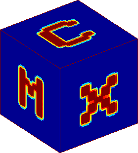
To create the above animation, we run 3 sequential simulations, projecting the "M", "C" and "X" patterns on 3 facets of the cube. Then we combine the 3 simulations and create the animation.
% the binary image of "MCX"
mcximg=[0 0 0 0 0 0 0 0 0 0 0
0 1 1 0 0 0 0 0 1 1 0
0 0 0 1 1 0 1 1 0 0 0
0 0 0 0 0 1 0 0 0 0 0
0 0 0 1 1 0 1 1 0 0 0
0 1 1 0 0 0 0 0 1 1 0
0 0 0 0 0 0 0 0 0 0 0
0 0 1 0 0 0 0 0 1 0 0
0 1 0 0 0 0 0 0 0 1 0
0 1 0 0 0 0 0 0 0 1 0
0 1 0 0 0 0 0 0 0 1 0
0 0 1 1 1 1 1 1 1 0 0
0 0 0 0 0 0 0 0 0 0 0
0 1 1 1 1 1 1 1 1 1 0
0 0 0 1 0 0 0 0 0 0 0
0 0 0 0 1 1 0 0 0 0 0
0 0 0 1 0 0 0 0 0 0 0
0 1 1 1 1 1 1 1 1 1 0
0 0 0 0 0 0 0 0 0 0 0];

cfg.nphoton=1e8;               % simulate 1e8 photons for each simulation
cfg.gpuid=1;                   % use the first GPU
cfg.autopilot=1;               % let mcx to determine thread numbers
cfg.tstart=0;                  % starting time
cfg.seed=99999;                % RNG seed

cfg.vol=uint8(ones(60,60,60)); % define the cubic volume
cfg.vol(25:35,25:35,25:35)=2;  % believe it or not, there is an inclusion
cfg.prop=[0 0 1 1;0.005 0.01 0.8 1.37;0.01 1,0.8,1.37]; % optical properties for 0,1,2, type 1 has very low scattering!
cfg.srctype='pattern';         % define an arbitrary pattern source
cfg.srcpattern=mcximg(1:6,:);  % take "X" first
cfg.srcpos=[-13 13 13];        % origin of the source
cfg.srcdir=[1 0 0];            % pointing in x direction
cfg.srcparam1=[0 30 0 size(cfg.srcpattern,1)]; % span 30x30 in y-z plane
cfg.srcparam2=[0 0 30 size(cfg.srcpattern,2)];
cfg.tend=0.3e-9;               % run it for 0.3 ns
cfg.tstep=0.1e-10;             % with 0.01 ns time gate, that's 30 gates
cfg.voidtime=0;                % start photon timer when entering the cube
flux=mcxlab(cfg);              % run the simulation
fcw1=flux.data*cfg.tstep;      % convert to fluence

cfg.srcpattern=rot90(mcximg(7:12,:),3);  % take the "C" pattern next
cfg.srcpos=[17 17 60+1];       % origin of the source
cfg.srcdir=[0 0 -1];           % shooting downward
cfg.srcparam1=[30 0 0 size(cfg.srcpattern,1)]; % the pattern spans 30x30 in x-y plane
cfg.srcparam2=[0 30 0 size(cfg.srcpattern,2)];
flux=mcxlab(cfg);              % run the second simulation
fcw2=flux.data*cfg.tstep;

cfg.srcpattern=mcximg(13:end,:); % take the "M" pattern last
cfg.srcpos=[60-15 -1 60-15];     % set source origin
cfg.srcdir=[0 1 0];              % pointing it in the y-axis
cfg.srcparam1=[-30 0 0 size(cfg.srcpattern,1)];  % spanning 30x30 in the x-z plane
cfg.srcparam2=[0 0 -30 size(cfg.srcpattern,2)];
flux=mcxlab(cfg);                % run the last simulation
fcw3=flux.data*cfg.tstep;

fcw=fcw1+fcw2+fcw3;              % sum 3 patterns, fcw has all 30 time gates

axis tight;                      % magics for making gif animations, blablabla
set(gca,'nextplot','replacechildren','visible','off');
set(gcf,'color','w');
dd=log10(abs(double(squeeze(fcw(:,:,:,1)))));
dd(isinf(dd))=-8;
hs=slice(dd,1,1,60);
set(hs,'linestyle','none');
axis equal; set(gca,'clim',[-6.5 -3])
box on;
set(gca,'xtick',[]);set(gca,'ytick',[]);set(gca,'ztick',[]);
drawnow;
fm = getframe;
[mcxframe,map] = rgb2ind(fm.cdata,256,'nodither');
mcxframe(1,1,1,size(fcw1,4)) = 0;
for i=1:size(fcw1,4)
    dd=log10(abs(double(squeeze(fcw(:,:,:,i)))));
    dd(isinf(dd))=-8;
    hs=slice(dd,1,1,60);
    set(hs,'linestyle','none');
    axis equal; set(gca,'clim',[-6.5 -3])
    set(gca,'xtick',[]);set(gca,'ytick',[]);set(gca,'ztick',[]);
    axis on;box on;
    drawnow;
    fm = getframe;
    mcxframe(:,:,1,i) = rgb2ind(fm.cdata,map,'nodither');
end
imwrite(mcxframe,map,'mcx_dice.gif','DelayTime',0.5,'LoopCount',inf);  % writing the gif file to disk, done!