The first feature allows users to define a scattering zenith angle distribution via a discretized inverse CDF (cumulative distribution function). The second feature allows users to define the zenith angle distribution for launching a photon, relative to the source-direction vector, also via a discretized inverse CDF. In MATLAB/Octave, they can be set as cfg.invcdf or cfg.angleinvcdf, respectively. We provided ready-to-use demo scripts in mcxlabcl/examples/demo_mcxlab_phasefun.m and demo_mcxlab_launchangle.m.

Additionally, in this release, we further improved the simulations when using Intel CPU or integrated GPU.

Aside from new features, a severe bug was discovered that affects all pattern and pattern3d simulations that do not use photon-sharing, please see

https://github.com/fangq/mcx/issues/212

Because of this bug, MCX/MCX-CL in older releases has been simulating squared pattern/pattern3d data instead of the pattern itself. If your simulation uses these two source types and you do not use photon-sharing (i.e. simulating multiple patterns together), please upgrade your MCX/MCX-CL and rerun your simulations. This bug only affect volumetric fluence/flux outputs; it does not affect diffuse reflectance outputs or binary patterns.

We also ported a bug fix from fangq/mcx#195 regarding precision loss when saving diffuse reflectance. Finally, starting from this release, we are providing native binary packages built for Apple M1/M2 (arm64) processors. All Apple silicon packages are labeled with macos-arm64 in the package names.

We want to thank Haohui Zhang for reporting a number of critical issues (fangq/mcx#195 and fangq/mcx#212). ShijieYan and fanyuyen have also contributed to the bug fixes and improvements.

The detailed updates can be found in the below change log

2024-03-12 [1fc8286] [ci] building binaries on Apple M1 macos-14 runner
2024-03-12 [bf89aff] [ci] update nightly build script
2024-03-08 [4891c72] [ci] remove mcxlabcl gcc warnings
2024-03-05 [80551a4] [bug] remove duplicated and overwritten cfg initialization
2024-03-04 [84c64ec] [bug] fix cuda core count for Ada and Blackwell
2024-03-01 [1e56f5b] [doc] update documentation for v2024.2
2024-03-01 [d4fb874] [ci] bump pmcxcl to v0.1.6
2024-03-01 [0d9f77f] [doc] update neurojson website url to https://neurojson.io
2024-02-29 [580cb27] [format] reformat all MATLAB codes with miss_hit
2024-02-29 [ce1d374] [bug] fixes to pass tests on Intel CPU, AMD GPU and pthread-AMD
2024-02-29 [2f70174] [bug] free ginvcdf and gangleinvcdf buffers
2024-02-29 [9aee8ce] [bug] fix many errors after testing, still need to fix replay
2024-02-29 [b82c856] [feat] add missing demo scripts
2024-02-29 [21e1e72]*[feat] port scattering and launch angle invcdf from fangq/mcx#129 fangq/mcx#13
2024-02-28 [90a28f3] [ci] remove macos-11 as brew fails for octave, Homebrew/brew#16209
2024-02-28 [fbe270b] [pmcxcl] bump pmcxcl to 0.1.4 after fixing fangq/mcx#212
2024-02-27 [4e1ec7f] [ci] fix windows cmake zlib error, fix mac libomp error
2024-02-27 [3d18b78]*[bug] fix critical bug, squaring pattern/pattern3d, fangq/mcx#212
2023-11-10 [26ec422] [ci] install mingw 8.1 for matlab mex build, matlab-actions/setup-matlab#75
2023-11-10 [5a96d02] [ci] set MW_MINGW64_LOC to octave bunded mingw, matlab-actions/setup-matlab#75
2023-10-31 [337c51c] [bug] apply fangq/mcx#195 fix to avoid dref accuracy loss
2023-10-29 [3b01475] further simplify bc handling, #47
2023-10-29 [f816140] latest matlab fails to respect MW_MINGW64_LOC on windows, use R2022a
2023-10-29 [adc0316] simplify boundary condition handling, fix #47
2023-10-07 [04a7155] bump pmcxcl to 0.1.3
2023-10-07 [e930448] remove opencl jit warnings, adjust optlevel order
2023-10-07 [1a30e5c] update copyright dates
2023-10-07 [dcdb117] fix unitinmm double-scaling bug, close #46, close #45
2023-10-03 [fa8dbb2] fix bc mcxlab/pmcxcl memory error,fangq/mcx#191,fangq/mcx#192
2023-09-29 [aa5da8c] fix -F flag overwrite bug
2023-09-26 [507b37b] fix continuous media scaling issue,pmcxcl 0.1.2, fangq/mcx#185
2023-09-26 [378f4eb] fix group load balancing for --optlevel 4
2023-09-24 [07bc297] additional patch to handle half-formatted cont. media

2. Introduction

Monte Carlo eXtreme (MCX) is a fast physically-accurate photon simulation software for 3D heterogeneous complex media. By taking advantage of the massively parallel threads and extremely low memory latency in a modern graphics processing unit (GPU), this program is able to perform Monte Carlo (MC) simulations at a blazing speed, typically hundreds to a thousand times faster than a single-threaded CPU-based MC implementation.

MCX-CL is the OpenCL implementation of the MCX algorithm. Unlike MCX which can only be executed on NVIDIA GPUs, MCX-CL is written in OpenCL, the Open Computing Language, and can be executed on most modern CPUs and GPUs available today, including Intel and AMD CPUs and GPUs. MCX-CL is highly portable, highly scalable and is feature-rich just like MCX.

Due to the nature of the underlying MC algorithms, MCX and MCX-CL are ray-tracing/ray-casting software under-the-hood. Compared to commonly seen ray-tracing libraries used in computer graphics or gaming engines, MCX-CL and MCX have many unique characteristics. The most important difference is that MCX/MCX-CL are rigorously based on physical laws. They are numerical solvers to the underlying radiative transfer equation (RTE) and their solutions have been validated across many publications using optical instruments and experimental measurements. In comparison, most graphics-oriented ray-tracers have to make many approximations in order to achieve fast rendering, enable to provide quantitatively accurate light simulation results. Because of this, MCX/MCX-CL have been extensively used by biophotonics research communities to obtain reference solutions and guide the development of novel medical imaging systems or clinical applications. Additionally, MCX/MCX-CL are volumetric ray-tracers; they traverse photon-rays throughout complex 3-D domains and computes physically meaningful quantities such as spatially resolved fluence, flux, diffuse reflectance/transmittance, energy deposition, partial pathlengths, among many others. In contrast, most graphics ray-tracing engines only trace the RGB color of a ray and render it on a flat 2-D screen. In other words, MCX/MCX-CL gives physically accurate 3-D light distributions while graphics ray-tracers focus on 2-D rendering of a scene at the camera. Nonetheless, they share many similarities, such as ray-marching computation, GPU acceleration, scattering/absorption handling etc.

The details of MCX-CL can be found in the below paper

[Yu2018] Leiming Yu, Fanny Nina-Paravecino, David Kaeli, and Qianqian Fang, "Scalable and massively parallel Monte Carlo photon transport simulations for heterogeneous computing platforms," J. Biomed. Optics, 23(1), 010504 (2018) .

A short summary of the main features includes:

3D heterogeneous media represented by voxelated array
support over a dozen source forms, including wide-field and pattern illuminations
boundary reflection support
time-resolved photon transport simulations
saving photon partial path lengths and trajectories
optimized random number generators
build-in flux/fluence normalization to output Green's functions
user adjustable voxel resolution
improved accuracy with atomic operations
cross-platform graphical user interface
native Matlab/Octave support for high usability
flexible JSON interface for future extensions
multi-GPU support
advanced features: photon-replay, photon-sharing, and more

MCX-CL can be used on Windows, Linux and Mac OS. Multiple user interfaces are provided, including

Command line mode: mcxcl can be executed in the command line, best suited for batch data processing
Graphical User Interface with MCXStudio: MCXStudio is a unified GUI program for MCX, MCX-CL and MMC. One can intuitively set all parameters, including GPU settings, MC settings and domain design, in the cross-platform interface
Calling inside MATLAB/Octave: mcxlabcl is a mex function, one can call it inside MATLAB or GNU Octave to get all functionalities as the command line version.
Calling inside Python: pmcxcl is a Python module wrapping the entire mcxcl simulation in an easy-to-use interface. One can install pmcxcl via pip install pmcxcl

If a user is familiar with MATLAB/Octave, it is highly recommended to use MCXCL in MATLAB/Octave to ease data visualization. If one prefers a GUI, please use MCXStudio to start. For users who are familiar with MCX/MCXCL and need it for regular data processing, using the command line mode is recommended.

3. Requirement and Installation

With the up-to-date driver installed for your computers, MCXCL can run on almost all computers. The requirements for using this software include

a modern CPU or GPU (Intel, NVIDIA, AMD, among others)
pre-installed graphics driver - typically includes the OpenCL runtime (libOpenCL.* or OpenCL.dll)

For speed differences between different CPUs/GPUs made by different vendors, please see your above paper [1] and our websites

Generally speaking, AMD and NVIDIA high-end dedicated GPUs perform the best, about 20-60x faster than a multi-core CPU; Intel's integrated GPU is about 3-4 times faster than a multi-core CPU.

MCX-CL supports and has been fully tested with open-source OpenCL runtime pocl (http://portablecl.org/) on the CPU. To install pocl, please run

  sudo apt-get install pocl-opencl-icd

To install MCXCL, you simply download the binary executable corresponding to your computer architecture and platform, extract the package and run the executable under the <mcxcl root>/bin directory. For Linux and MacOS users, please double check and make sure libOpenCL.so is installed under the /usr/lib directory. If it is installed under a different directory, please define environment variable LD_LIBRARY_PATH to include the path.

If libOpenCL.so or OpenCL.dll does not exist on your system or, please make sure you have installed CUDA SDK (if you are using an nVidia card) or AMD APP SDK (if you are using an AMD card).

The below installation steps can be browsed online at

https://mcx.space/wiki/index.cgi/wiki/index.cgi?Workshop/MCX18Preparation/MethodA

3.1. Step 1. Verify your CPU/GPU support

MCX-CL supports a wide-range of processors, including Intel/AMD CPUs and GPUs from NVIDIA/AMD/Intel. If your computer has been working previously, in most cases, MCX-CL can simply run out-of-box. However, if you have trouble, please follow the below detailed steps to verify and setup your OS to run MCX-CL.

3.1.1. Verify GPU/CPU support

To verify if you have installed the OpenCL or CUDA support, you may

if you have a windows machine, download and install the Everything Search tool (a small and fast file name search utility), and type "opencl.dll" in the search bar
- Expected result: you must see OpenCL.dll (or nvopencl.dll if you have an NVIDIA GPU) installed in the Windows\System32 directory.
if you have an Mac, open a terminal, and type ls /System/Library/Frameworks/OpenCL.framework/Versions/A/OpenCL
- Expected result: you should not see an error.
if you have a Linux laptop, open a terminal, and type locate libOpenCL.so,
- Expected result: you should see one or multiple libOpenCL files

If the OpenCL.dll file is not found on your system, please read the below sections. Otherwise, please go to Step 2: Install MATLAB.

3.1.2. Computers without discrete GPUs

In many cases, your computer runs on an Intel CPU with integrated graphics. In this case, please make sure you have installed the latest Intel graphics drivers. If you are certain that you have installed the graphics drivers, or your graphics works smoothly, please skip this step.

If you want to double check, for Windows machine, you can download the "Intel Driver&Support Assistant" to check if you have installed the graphics drivers

https://downloadcenter.intel.com/download/24345/Intel-Driver-Support-Assistant

for a Mac, you need to use your App store to update the driver, see the below link for details

https://www.intel.com/content/www/us/en/support/articles/000022440/graphics-drivers.html

for a Linux (for example Ubuntu) laptop, the intel CPU OpenCL run-time can be downloaded from

https://software.intel.com/en-us/articles/opencl-drivers#latest_CPU_runtime

if you want to use both Intel CPU and GPU on Linux, you need to install the OpenCL™ 2.0 GPU/CPU driver package for Linux* (this involves compiling a new kernel)

https://software.intel.com/en-us/articles/opencl-drivers#latest_linux_driver

3.1.3. Computers with discrete GPUs

If you have a computer with a discrete GPU, you need to make sure your discrete GPU is configured with the appropriate GPU driver installed. Again, if you have been using your laptop regularly and the graphics has been smooth, likely your graphics driver has already been installed.

If your GPU driver was not installed, and would like to install, or upgrade from an older version, for an NVIDIA GPU, you may browse this link to install the matching driver

http://www.nvidia.com/Download/index.aspx

if your GPU is an AMD GPU, please use the below link

https://support.amd.com/en-us/download

It is also possible to simultaneously access Intel CPU along with your discrete GPU. In this case, you need to download the latest Intel OpenCL Runtime for CPU only if you haven't installed it already.

https://software.intel.com/en-us/articles/opencl-drivers#latest_CPU_runtime

Note: if you have an NVIDIA GPU, there is no need to install CUDA in order for you to run MCX-CL/MCXLABCL.

3.1.4. Computers with hybrid GPUs

We noticed that running Ubuntu Linux 22.04 with a 6.5 kernel on a laptop with a hybrid GPU with an Intel iGPU and an NVIDIA GPU, you must configure the laptop to use the NVIDIA GPU as the primary GPU by choosing "NVIDIA (Performance Mode)" in the PRIME Profiles section of **NVIDIA X Server Settings**. You can also run

    sudo prime-select nvidia

to achieve the same goal. Otherwise, the simulation may hang your system after running for a few seconds. A hybrid GPU laptop combing an NVIDIA GPU with an AMD iGPU does not seem to have this issue if using Linux.

In addition, NVIDIA drirver (520 or newer) has a known glitch running on Linux kernel 6.x (such as those in Ubuntu 22.04). See

https://forums.developer.nvidia.com/t/dev-nvidia-uvm-io-error-on-ubuntu-22-04-520-to-535-driver-versions/262153

When the laptop is in the "performance" mode and wakes up from suspension, MCX/MCX-CL/MMC or any CUDA program fails to run with an error

    MCX ERROR(-999):unknown error in unit mcx_core.cu:2523

This is because the kernel module nvida-uvm fails to be reloaded after suspension. If you had an open MATLAB session, you must close MATLAB first, and run the below commands (if MATLAB is open, you will see rmmod: ERROR: Module nvidia_uvm is in use)

    sudo rmmod /dev/nvidia-uvm
    sudo modprobe nvidia-uvm

after the above command, MCX-CL should be able to run again.

3.2. Step 2. Install MATLAB or GNU Octave

One must install either a MATLAB or GNU Octave if one needs to use mcxlabcl. If you use a Mac or Linux laptop, you need to create a link (if this link does not exist) so that your system can find MATLAB. To do this you start a terminal, and type

 sudo ln -s /path/to/matlab /usr/local/bin

please replace /path/to/matlab to the actual matlab command full path (for Mac, this is typically /Application/MATLAB_R20???.app/bin/matlab, for Linux, it is typically /usr/local/MATLAB/R20???/bin/matlab, ??? is the year and release, such as 18a, 17b etc). You need to type your password to create this link.

To verify your computer has MATLAB installed, please start a terminal on a Mac or Linux, or type "cmd" and enter in Windows start menu, in the terminal, type "matlab" and enter, you should see MATLAB starts.

3.3. Step 3. Download MCXCL

One can download two separate MCXCL packages (standalone mcxcl binary, and mcxlabcl) or download the integrated MCXStudio package (which contains mcx, mcxcl, mmc, mcxlab, mcxlabcl and mmclab) where both packages, and many more, are included. The latest stable released can be found on the MCX's website. However, if you want to use the latest (but sometimes containing half-implemented features) software, you can access the nightly-built packages from

https://mcx.space/nightly/

If one has downloaded the mcxcl binary package, after extraction, you may open a terminal (on Windows, type cmd the Start menu), cd mcxcl folder and then cd the bin subfolder. Please type "mcxcl" and enter, if the binary is compatible with your OS, you should see the printed help info. The next step is to run

 mcxcl -L

this will query your system and find any hardware that can run mcxcl. If your hardware (CPU and GPU) have proper driver installed, the above command will typically return 1 or more available computing hardware. Then you can move to the next step.

If you do not see any processor printed, that means your CPU or GPU does not have OpenCL support (because it is too old or no driver installed). You will need to go to their vendor's website and download the latest driver. For Intel CPUs older than Ivy Bridge (4xxx), OpenCL and MCXCl are not well supported. Please consider installing dedicated GPU or use a different computer.

In the case one has installed the MCXStudio package, you may follow the below procedure to test for hardware compatibility.

Please click on the folder matching your operating system (for example, if you run a 64bit Windows, you need to navigate into win64 folder), and download the file named "MCXStudio-MCX18-nightlybuild.zip".

Open this file, and unzip it to a working folder (for Windows, for example, the Documents or Downloads folder). The package needs about 100 MB disk space.

Once unzipped, you should be able to see a folder named "MCXStudio", with a few executables and 3 subfolders underneath. See the folder structure below:

MCXStudio/
├── MATLAB/
│   ├── mcxlab/
│   ├── mcxlabcl/
│   └── mmclab/
├── MCXSuite/
│   ├── mcx/
│   ├── mcxcl/
│   └── mmc/
├── mcxstudio
├── mcxshow
└── mcxviewer

Please make sure that your downloaded MCXStudio must match your operating system.

3.3.1. Notes for Mac Users

For Mac users: Please unzip the package under your home directory directly (Shift+Command+H).

3.3.2. Notes for Windows Users

When you start MCXStudio, you may see a dialog to ask you to modify the TdrDelay key in the registry so that mcx can run more than 5 seconds. If you select Yes, some of you may get an error saying you do not have permission.

To solve this problem, you need to quit MCXStudio, and then right-click on the mcxstudio.exe, and select "Run as Administrator". Then, you should be able to apply the registry change successfully.

Alternatively, one should open file browser, navigate into mcxcl/setup/win64 folder, and right-click on the "apply_timeout_registry_fix.bat" file and select "Run as Administrator".

You must reboot your computer for this change to be effective!

3.4. Step 4. Start MCXStudio and query GPU information

Now, navigate to the MCXStudio folder (i.e. the top folder of the extracted software structure). On Windows, right-click on the executable named "mcxstudio.exe" and select "Run as Administrator" for the first time only; on the Linux, double click on the mcxstudio executable; on the Mac, open a terminal and type

 cd ~/MCXStudio
 open mcxstudio.app

First, click on the "New" button to the top-left (green plus icon), select the 3rd option "NVIDIA/AMD/Intel CPUs/GPUs (MCX-CL)", and type a session name "test" in the field below. Then click OK. You should see a blue/yellow "test" icon added to the left panel.

Now, click on the "GPU" button on the toolbar (6th button from the left side), an Output window will popup, and wait for a few seconds, you should see an output like

"-- Run Command --"
"mcxcl" -L
"-- Printing GPU Information --"
Platform [0] Name NVIDIA CUDA
============ GPU device ID 0 [1 of 2]: Graphics Device  ============
 Device 1 of 2:		Graphics Device
 Compute units   :	80 core(s)
 Global memory   :	12644188160 B
 Local memory    :	49152 B
 Constant memory :	65536 B
 Clock speed     :	1455 MHz
 Compute Capacity:	7.0
 Stream Processor:	10240
 Vendor name    :	NVIDIA
 Auto-thread    :	655360       
...
Platform [1] Name Intel(R) OpenCL
============ CPU device ID 2 [1 of 1]: Intel(R) Core(TM) i7-7700K CPU @ 4.20GHz  ============
 Device 3 of 1:		Intel(R) Core(TM) i7-7700K CPU @ 4.20GHz
 Compute units   :	8 core(s)
 Global memory   :	33404575744 B
 Local memory    :	32768 B
 Constant memory :	131072 B
 Clock speed     :	4200 MHz
 Vendor name    :	Intel
 Auto-thread    :	512
 Auto-block     :	64

"-- Task completed --"

Your output may look different from above. If you do not see any output, or it returns no GPU found, that means your OpenCL support was not installed properly. Please go back to Steps 1-2 and reinstall the drivers.

If you have Intel CPU with Integrated GPU, you should be able to see a section with "Platform [?] Name Intel(R) OpenCL" in the above output. You may see only the CPU is listed, or both the CPU and the integrated GPU.

3.5. Step 5. Run a trial simulation

If your above GPU query was successful, you should now see in the middle panel of the MCXStudio window, under the Section entitled "GPU Settings", in a check-box list under "Run MCX on", you should now see the available devices on your laptop.

To avoid running lengthy simulations, please change the "Total photon number (-n)" field under the "Basic Settings" from 1e6 to 1e5.

Now, you can then run a trial simulation, by first clicking on the "Validate" button (blue check-mark icon), and then click on "Run" (the button to the right of validate). This will launch an MCXCL simulation. The output window will show again, and you can see the messages printed from the simulation, similar to the output below

"-- Command: --"
mcxcl --session "preptest"  --input "/drives/taote1/users/fangq/Download/MCXStudio/Output/mcxclsessions/preptest/preptest.json" --root "/drives/taote1/users/fangq/Download/MCXStudio/Output/mcxclsessions/preptest" --outputformat mc2 --gpu 10 --autopilot 1 --photon 10000000 --normalize 1 --save2pt 1 --reflect 1 --savedet 1 --unitinmm 1.00 --saveseed 0 --seed "1648335518" --compileropt "-D USE_ATOMIC" --array 0 --dumpmask 0 --repeat 1  --maxdetphoton 10000000
"-- Executing Simulation --"
==============================================================================
=                       Monte Carlo eXtreme (MCX) -- OpenCL                  =
=          Copyright (c) 2010-2024 Qianqian Fang <q.fang at neu.edu>         =
=                https://mcx.space/  &  https://neurojson.io/                =
=                                                                            =
= Computational Optics&Translational Imaging (COTI) Lab - http://fanglab.org =
=   Department of Bioengineering, Northeastern University, Boston, MA, USA   =
==============================================================================
=    The MCX Project is funded by the NIH/NIGMS under grant R01-GM114365     =
==============================================================================
= Open-source codes and reusable scientific data are essential for research, =
= MCX proudly developed human-readable JSON-based data formats for easy reuse=
=                                                                            =
=Please visit our free scientific data sharing portal at https://neurojson.io=
= and consider sharing your public datasets in standardized JSON/JData format =
==============================================================================
$Rev::4fdc45$v2024.2 $Date::2018-03-29 00:35:53 -04$by $Author::Qianqian Fang$
==============================================================================
- variant name: [Detective MCXCL] compiled with OpenCL version [1]
- compiled with: [RNG] Logistic-Lattice [Seed Length] 5
initializing streams ...	init complete : 0 ms

Building kernel with option: -cl-mad-enable -DMCX_USE_NATIVE -DMCX_SIMPLIFY_BRANCH -DMCX_VECTOR_INDEX -DMCX_SRC_PENCIL  -D USE_ATOMIC -DUSE_ATOMIC -D MCX_SAVE_DETECTORS -D MCX_DO_REFLECTION
build program complete : 23 ms
- [device 0(1): Graphics Device] threadph=15 oddphotons=169600 np=10000000.0 nthread=655360 nblock=64 repetition=1
set kernel arguments complete : 23 ms
lauching mcx_main_loop for time window [0.0ns 5.0ns] ...
simulation run# 1 ... 

kernel complete:  	796 ms
retrieving flux ... 	
detected 0 photons, total: 0	transfer complete:        818 ms
normalizing raw data ...	normalization factor alpha=20.000000
saving data to file ... 216000 1	saving data complete : 821 ms

simulated 10000000 photons (10000000) with 1 devices (repeat x1)
MCX simulation speed: 12953.37 photon/ms
total simulated energy: 10000000.00	absorbed: 27.22654%
(loss due to initial specular reflection is excluded in the total)

If this simulation is completed successfully, you should be able to see the "Simulation speed" and total simulated energy reported at the end. Please verify your "absorbed" percentage value printed at the end (in bold above), and make sure it is ~27%. We found that some Intel OpenCL library versions produced incorrect results.

If your laptop shows an error for the Intel GPU, please choose another device from the "GPU Settings" section, and run the simulation again.

If your GPU/CPU gives the below error (found on HD4400 GPU and 4th gen Intel CPUs)

  error: OpenCL extension 'cl_khr_fp64' is unsupported
  MCXCL ERROR(11):Error: Failed to build program executable! in unit mcx_host.cpp:510

You may add

   -J "-DUSE_LL5_RAND"

in the MCXStudio GUI\Advanced Settings\Additional Parameters field. This should allow it to run, but please verify the absorption fraction is ~27%. For 4th generation Intel CPU, we found that install the Intel CPU OpenCL run-time can produce correct simulations. Please download it from here

https://software.intel.com/en-us/articles/opencl-drivers#latest_CPU_runtime

3.6. Step 6. Test MATLAB for visualization

From v2019.3, MCXStudio provides builtin 3D volume visualization, this step is no longer needed.

3.7. Step 7. Setting up MATLAB search path

The next step is to set up the search paths for MCXLAB/MMCLAB. You need to start MATLAB, and in the Command window, please type

 pathtool

this will popup a window. Click on the "Add with Subfolders ..." button (the 2nd from the top), then browse the MCXStudio folder, then select OK. Now you should see all needed MCX/MMC paths are added to MATLAB. Before you quick this window, click on the "Save" button.

To verify if your MCXLAB/MMCLAB/MCXLABCL has been installed properly, please type

 which mcxlab
 which mmclab
 which mcxlabcl

you should see their full paths printed.

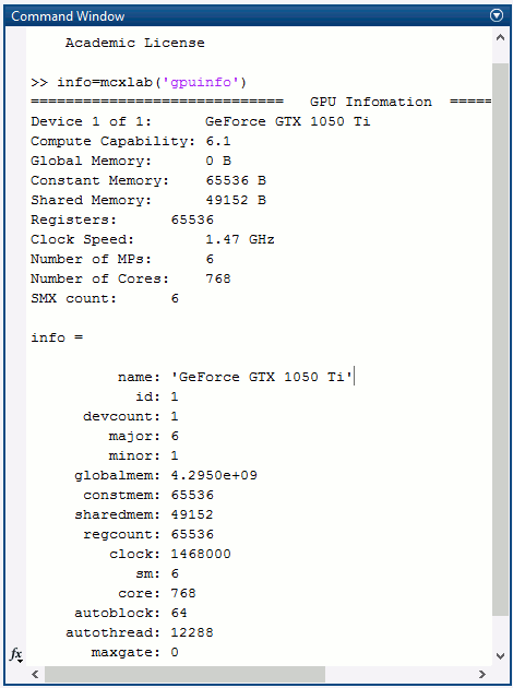
To see if you can run MCXLAB-CL in your environment, please type

 USE_MCXCL=1   %define this line in the base workspace, all subsequent mcxlab calls will use mcxcl
 info=mcxlab('gpuinfo')
 clear USE_MCXCL

this should print a list of CPU/GPU devices using which you can run the MC simulations.

If you do not see any output, that means your CPU/GPU OpenCL driver was not installed properly, you need to go back to Steps 1-2.

If you have an NVIDIA GPU, and have installed the proper GPU driver, you may run

 info=mcxlab('gpuinfo')  % notice the command is mcxlab instead of mcxlabcl

this should print a list of NVIDIA GPU from the MATLAB window.

4. Running Simulations

To run a simulation, the minimum input is a configuration (text) file, and a volume (a binary file with each byte representing a medium index). Typing the name of the executable without any parameters, will print the help information and a list of supported parameters, such as the following:

==============================================================================
=                       Monte Carlo eXtreme (MCX) -- OpenCL                  =
=          Copyright (c) 2010-2024 Qianqian Fang <q.fang at neu.edu>         =
=                https://mcx.space/  &  https://neurojson.io/                =
=                                                                            =
= Computational Optics&Translational Imaging (COTI) Lab - http://fanglab.org =
=   Department of Bioengineering, Northeastern University, Boston, MA, USA   =
==============================================================================
=    The MCX Project is funded by the NIH/NIGMS under grant R01-GM114365     =
==============================================================================
= Open-source codes and reusable scientific data are essential for research, =
= MCX proudly developed human-readable JSON-based data formats for easy reuse=
=                                                                            =
=Please visit our free scientific data sharing portal at https://neurojson.io=
= and consider sharing your public datasets in standardized JSON/JData format =
==============================================================================
$Rev::4fdc45$v2024.2 $Date::2018-03-29 00:35:53 -04$by $Author::Qianqian Fang$
==============================================================================

usage: mcxcl <param1> <param2> ...
where possible parameters include (the first value in [*|*] is the default)

== Required option ==
 -f config     (--input)       read an input file in .json or .inp format
                               if the string starts with '{', it is parsed as
			       an inline JSON input file
      or
 --bench ['cube60','skinvessel',..] run a buint-in benchmark specified by name
                               run --bench without parameter to get a list

== MC options ==
 -n [0|int]    (--photon)      total photon number (exponential form accepted)
 -r [1|+/-int] (--repeat)      if positive, repeat by r times,total= #photon*r
                               if negative, divide #photon into r subsets
 -b [1|0]      (--reflect)     1 to reflect photons at ext. boundary;0 to exit
 -B '______'   (--bc)          per-face boundary condition (BC), 6 letters for
    /case insensitive/         bounding box faces at -x,-y,-z,+x,+y,+z axes;
			       overwrite -b if given. 
			       each letter can be one of the following:
			       '_': undefined, fallback to -b
			       'r': like -b 1, Fresnel reflection BC
			       'a': like -b 0, total absorption BC
			       'm': mirror or total reflection BC
			       'c': cyclic BC, enter from opposite face

			       if input contains additional 6 letters,
			       the 7th-12th letters can be:
			       '0': do not use this face to detect photon, or
			       '1': use this face for photon detection (-d 1)
			       the order of the faces for letters 7-12 is 
			       the same as the first 6 letters
			       eg: --bc ______010 saves photons exiting at y=0
 -u [1.|float] (--unitinmm)    defines the length unit for the grid edge
 -U [1|0]      (--normalize)   1 to normalize flux to unitary; 0 save raw
 -E [0|int|.jdat] (--seed)     set random-number-generator seed, -1 to generate
                               if a jdat/mch file is followed, MCX "replays" 
                               the detected photon; the replay mode can be used
                               to calculate the mua/mus Jacobian matrices
 -z [0|1]      (--srcfrom0)    1 volume origin is [0 0 0]; 0: origin at [1 1 1]
 -Y [0|int]    (--replaydet)   replay only the detected photons from a given 
                               detector (det ID starts from 1), used with -E 
			       if 0, replay all detectors and sum all Jacobians
			       if -1, replay all detectors and save separately
 -V [0|1]      (--specular)    1 source located in the background,0 inside mesh
 -e [0.|float] (--minenergy)   minimum energy level to trigger Russian roulette
 -g [1|int]    (--gategroup)   number of maximum time gates per run

== GPU options ==
 -L            (--listgpu)     print GPU information only
 -t [16384|int](--thread)      total thread number
 -T [64|int]   (--blocksize)   thread number per block
 -A [1|int]    (--autopilot)   auto thread config:1 enable;0 disable
 -G [0|int]    (--gpu)         specify which GPU to use, list GPU by -L; 0 auto
      or
 -G '1101'     (--gpu)         using multiple devices (1 enable, 0 disable)
 -W '50,30,20' (--workload)    workload for active devices; normalized by sum
 -I            (--printgpu)    print GPU information and run program
 -o [1|int]    (--optlevel)    optimization level 0-no opt;1,2,3 more optimized
 -J '-DMACRO'  (--compileropt) specify additional JIT compiler options
                               A few built-in preprocessors include
              -DMCX_GPU_DEBUG  - print step-by-step debug info
 -k my_simu.cl (--kernel)      user specified OpenCL kernel source file

== Input options ==
 -P '{...}'    (--shapes)      a JSON string for additional shapes in the grid.
                               only the root object named 'Shapes' is parsed 
			       and added to the existing domain defined via -f 
			       or --bench
 -j '{...}'    (--json)        a JSON string for modifying all input settings.
                               this input can be used to modify all existing 
			       settings defined by -f or --bench
 -K [1|int|str](--mediabyte)   volume data format, use either a number or a str
                               1 or byte: 0-128 tissue labels
			       2 or short: 0-65535 (max to 4000) tissue labels
			       4 or integer: integer tissue labels 
                             100 or muamus_float: 2x 32bit floats for mua/mus
                             101 or mua_float: 1 float per voxel for mua
			     102 or muamus_half: 2x 16bit float for mua/mus
			     103 or asgn_byte: 4x byte gray-levels for mua/s/g/n
			     104 or muamus_short: 2x short gray-levels for mua/s
 -a [0|1]      (--array)       1 for C array (row-major); 0 for Matlab array

== Output options ==
 -s sessionid  (--session)     a string to label all output file names
 -O [X|XFEJPML](--outputtype)  X - output flux, F - fluence, E - energy density
                               J - Jacobian (replay mode),   P - scattering
                               event counts at each voxel (replay mode only)
                               M - momentum transfer; L - total pathlength
 -d [1|0-3]    (--savedet)     1 to save photon info at detectors; 0 not save
                               2 reserved, 3 terminate simulation when detected
                               photon buffer is filled
 -w [DP|DSPMXVW](--savedetflag)a string controlling detected photon data fields
    /case insensitive/         1 D  output detector ID (1)
                               2 S  output partial scat. even counts (#media)
                               4 P  output partial path-lengths (#media)
			       8 M  output momentum transfer (#media)
			      16 X  output exit position (3)
			      32 V  output exit direction (3)
			      64 W  output initial weight (1)
      combine multiple items by using a string, or add selected numbers together
      by default, mcx only saves detector ID and partial-path data
 -x [0|1]      (--saveexit)    1 to save photon exit positions and directions
                               setting -x to 1 also implies setting '-d' to 1
			       same as adding 'XV' to -w.
 -X [0|1]      (--saveref)     1 to save diffuse reflectance at the air-voxels
                               right outside of the domain; if non-zero voxels
			       appear at the boundary, pad 0s before using -X
 -m [0|1]      (--momentum)    1 to save photon momentum transfer,0 not to save.
                               same as adding 'M' to the -w flag
 -q [0|1]      (--saveseed)    1 to save photon RNG seed for replay; 0 not save
 -M [0|1]      (--dumpmask)    1 to dump detector volume masks; 0 do not save
 -H [1000000] (--maxdetphoton) max number of detected photons
 -S [1|0]      (--save2pt)     1 to save the flux field; 0 do not save
 -F [jnii|...](--outputformat) fluence data output format:
                               mc2 - MCX mc2 format (binary 32bit float)
                               jnii - JNIfTI format (https://neurojson.org)
                               bnii - Binary JNIfTI (https://neurojson.org)
                               nii - NIfTI format
                               hdr - Analyze 7.5 hdr/img format
                               tx3 - GL texture data for rendering (GL_RGBA32F)
	the bnii/jnii formats support compression (-Z) and generate small files
	load jnii (JSON) and bnii (UBJSON) files using below lightweight libs:
	  MATLAB/Octave: JNIfTI toolbox   https://github.com/NeuroJSON/jnifti, 
	  MATLAB/Octave: JSONLab toolbox  https://github.com/NeuroJSON/jsonlab,
	  Python:        PyJData:         https://pypi.org/project/jdata
	  JavaScript:    JSData:          https://github.com/NeuroJSON/jsdata
 -Z [zlib|...] (--zip)         set compression method if -F jnii or --dumpjson
                               is used (when saving data to JSON/JNIfTI format)
			       0 zlib: zip format (moderate compression,fast) 
			       1 gzip: gzip format (compatible with *.gz)
			       2 base64: base64 encoding with no compression
			       3 lzip: lzip format (high compression,very slow)
			       4 lzma: lzma format (high compression,very slow)
			       5 lz4: LZ4 format (low compression,extrem. fast)
			       6 lz4hc: LZ4HC format (moderate compression,fast)
 --dumpjson [-,0,1,'file.json']  export all settings,including volume data using
                               JSON/JData (https://neurojson.org) format for
			       easy sharing; can be reused using -f
			       if followed by nothing or '-', mcx will print
			       the JSON to the console; write to a file if file
			       name is specified; by default, prints settings
			       after pre-processing; '--dumpjson 2' prints 
			       raw inputs before pre-processing

== User IO options ==
 -h            (--help)        print this message
 -v            (--version)     print MCX revision number
 -l            (--log)         print messages to a log file instead
 -i 	       (--interactive) interactive mode

== Debug options ==
 -D [0|int]    (--debug)       print debug information (you can use an integer
  or                           or a string by combining the following flags)
 -D [''|RMPT]                  1 R  debug RNG
    /case insensitive/         2 M  store photon trajectory info
                               4 P  print progress bar
                               8 T  save trajectory data only, disable flux/detp
      combine multiple items by using a string, or add selected numbers together

== Additional options ==
 --atomic       [1|0]          1: use atomic operations; 0: do not use atomics
 --voidtime     [1|0]          when src is outside, 1 enables timer inside void
 --showkernel   [1|0]          1:display the default or loaded (-k) MCXCL kernel
 --root         [''|string]    full path to the folder storing the input files
 --internalsrc  [0|1]          set to 1 to skip entry search to speedup launch
 --gscatter     [1e9|int]      after a photon completes the specified number of
                               scattering events, mcx then ignores anisotropy g
                               and only performs isotropic scattering for speed
 --maxvoidstep  [1000|int]     maximum distance (in voxel unit) of a photon that
                               can travel before entering the domain, if 
                               launched outside (i.e. a widefield source)
 --maxjumpdebug [10000000|int] when trajectory is requested (i.e. -D M),
                               use this parameter to set the maximum positions
                               stored (default: 1e7)

== Example ==
example: (list built-in benchmarks)
       mcxcl --bench
or (list supported GPUs on the system)
       mcxcl -L
or (use multiple devices - 1st,2nd and 4th GPUs - together with equal load)
       mcxcl --bench cube60b -n 1e7 -G 1101 -W 10,10,10
or (use inline domain definition)
       mcxcl -f input.json -P '{"Shapes":[{"ZLayers":[[1,10,1],[11,30,2],[31,60,3]]}]}'
or (use inline json setting modifier)
       mcxcl -f input.json -j '{"Optode":{"Source":{"Type":"isotropic"}}}'
or (dump simulation in a single json file)
       mcxcl --bench cube60planar --dumpjson

To further illustrate the command line options, below one can find a sample command

  mcxcl -A 0 -t 16384 -T 64 -n 1e7 -G 1 -f input.json -r 2 -s test -g 10 -d 1 -w dpx -b 1

the command above asks mcxcl to manually (-A 0) set GPU threads, and launch 16384 GPU threads (-t) with every 64 threads a block (-T); a total of 1e7 photons (-n) are simulated by the first GPU (-G 1) and repeat twice (-r) - i.e. total 2e7 photons; the media/source configuration will be read from a JSON file named input.json (-f) and the output will be labeled with the session id “test” (-s); the simulation will run 10 concurrent time gates (-g) if the GPU memory can not simulate all desired time gates at once. Photons passing through the defined detector positions are saved for later rescaling (-d); refractive index mismatch is considered at media boundaries (-b).

Historically, MCXCL supports an extended version of the input file format (.inp) used by tMCimg. However, we are phasing out the .inp support and strongly encourage users to adopt JSON formatted (.json) input files. Many of the advanced MCX options are only supported in the JSON input format.

1000000              # total photon, use -n to overwrite in the command line
29012392             # RNG seed, negative to generate, use -E to overwrite
30.0 30.0 0.0 1      # source position (in grid unit), the last num (optional) sets --srcfrom0 (-z)
0 0 1 0              # initial directional vector, 4th number is the focal-length, 0 for collimated beam, nan for isotropic
0.e+00 1.e-09 1.e-10 # time-gates(s): start, end, step
semi60x60x60.bin     # volume ('unsigned char' binary format, or specified by -K/--mediabyte)
1 60 1 60            # x voxel size in mm (isotropic only), dim, start/end indices
1 60 1 60            # y voxel size, must be same as x, dim, start/end indices 
1 60 1 60            # y voxel size, must be same as x, dim, start/end indices
1                    # num of media
1.010101 0.01 0.005 1.37  # scat. mus (1/mm), g, mua (1/mm), n
4       1.0          # detector number and default radius (in grid unit)
30.0  20.0  0.0  2.0 # detector 1 position (real numbers in grid unit) and individual radius (optional)
30.0  40.0  0.0      # ..., if individual radius is ignored, MCX will use the default radius
20.0  30.0  0.0      #
40.0  30.0  0.0      # 
pencil               # source type (optional)
0 0 0 0              # parameters (4 floats) for the selected source
0 0 0 0              # additional source parameters

Note that the scattering coefficient mus=musp/(1-g).

The volume file (semi60x60x60.bin in the above example), can be read in two ways by MCX: row-major[3] or column-major depending on the value of the user parameter -a. If the volume file was saved using matlab or fortran, the byte order is column-major, and you should use -a 0 or leave it out of the command line. If it was saved using the fwrite() in C, the order is row-major, and you can either use -a 1.

You may replace the binary volume file by a JSON-formatted shape file. Please refer to Section V for details.

The time gate parameter is specified by three numbers: start time, end time and time step size (in seconds). In the above example, the configuration specifies a total time window of [0 1] ns, with a 0.1 ns resolution. That means the total number of time gates is 10.

MCXCL provides an advanced option, -g, to run simulations when the GPU memory is limited. It specifies how many time gates to simulate concurrently. Users may want to limit that number to less than the total number specified in the input file - and by default it runs one gate at a time in a single simulation. But if there's enough memory based on the memory requirement in Section II, you can simulate all 10 time gates (from the above example) concurrently by using "-g 10" in which case you have to make sure the video card has at least 60*60*60*10*5=10MB of free memory. If you do not include the -g, MCX will assume you want to simulate just 1 time gate at a time.. If you specify a time-gate number greater than the total number in the input file, (e.g, "-g 20") MCX will stop when the 10 time-gates are completed. If you use the autopilot mode (-A), then the time-gates are automatically estimated for you.

5. Using JSON-formatted input files

Starting from version 0.7.9, MCX accepts a JSON-formatted input file in addition to the conventional tMCimg-like input format. JSON (JavaScript Object Notation) is a portable, human-readable and “fat-free” text format to represent complex and hierarchical data. Using the JSON format makes a input file self-explanatory, extensible and easy-to-interface with other applications (like MATLAB).

A sample JSON input file can be found under the examples/quicktest folder. The same file, qtest.json, is also shown below:

{
    "Help": {
      "[en]": {
        "Domain::VolumeFile": "file full path to the volume description file, can be a binary or JSON file",
        "Domain::Dim": "dimension of the data array stored in the volume file",
        "Domain::OriginType": "similar to --srcfrom0, 1 if the origin is [0 0 0], 0 if it is [1.0,1.0,1.0]",
	"Domain::LengthUnit": "define the voxel length in mm, similar to --unitinmm",
        "Domain::Media": "the first medium is always assigned to voxels with a value of 0 or outside of
                         the volume, the second row is for medium type 1, and so on. mua and mus must 
                         be in 1/mm unit",
        "Session::Photons": "if -n is not specified in the command line, this defines the total photon number",
        "Session::ID": "if -s is not specified in the command line, this defines the output file name stub",
        "Forward::T0": "the start time of the simulation, in seconds",
        "Forward::T1": "the end time of the simulation, in seconds",
        "Forward::Dt": "the width of each time window, in seconds",
        "Optode::Source::Pos": "the grid position of the source, can be non-integers, in grid unit",
        "Optode::Detector::Pos": "the grid position of a detector, can be non-integers, in grid unit",
        "Optode::Source::Dir": "the unitary directional vector of the photon at launch",
        "Optode::Source::Type": "source types, must be one of the following: 
                   pencil,isotropic,cone,gaussian,planar,pattern,fourier,arcsine,disk,fourierx,fourierx2d,
		   zgaussian,line,slit,pencilarray,pattern3d",
        "Optode::Source::Param1": "source parameters, 4 floating-point numbers",
        "Optode::Source::Param2": "additional source parameters, 4 floating-point numbers"
      }
    },
    "Domain": {
	"VolumeFile": "semi60x60x60.bin",
        "Dim":    [60,60,60],
        "OriginType": 1,
	"LengthUnit": 1,
        "Media": [
             {"mua": 0.00, "mus": 0.0, "g": 1.00, "n": 1.0},
             {"mua": 0.005,"mus": 1.0, "g": 0.01, "n": 1.0}
        ]
    },
    "Session": {
	"Photons":  1000000,
	"RNGSeed":  29012392,
	"ID":       "qtest"
    },
    "Forward": {
	"T0": 0.0e+00,
	"T1": 5.0e-09,
	"Dt": 5.0e-09
    },
    "Optode": {
	"Source": {
	    "Pos": [29.0, 29.0, 0.0],
	    "Dir": [0.0, 0.0, 1.0],
	    "Type": "pencil",
	    "Param1": [0.0, 0.0, 0.0, 0.0],
	    "Param2": [0.0, 0.0, 0.0, 0.0]
	},
	"Detector": [
	    {
		"Pos": [29.0,  19.0,  0.0],
		"R": 1.0
	    },
            {
                "Pos": [29.0,  39.0,  0.0],
                "R": 1.0
            },
            {
                "Pos": [19.0,  29.0,  0.0],
                "R": 1.0
            },
            {
                "Pos": [39.0,  29.0,  0.0],
                "R": 1.0
            }
	]
    }
}

A JSON input file requiers several root objects, namely "Domain", "Session", "Forward" and "Optode". Other root sections, like "Help", will be ignored. Each object is a data structure providing information indicated by its name. Each object can contain various sub-fields. The orders of the fields in the same level are flexible. For each field, you can always find the equivalent fields in the *.inp input files. For example, The "VolumeFile" field under the "Domain" object is the same as Line#6 in qtest.inp; the "RNGSeed" under "Session" is the same as Line#2; the "Optode.Source.Pos" is the same as the triplet in Line#3; the "Forward.T0" is the same as the first number in Line#5, etc.

An MCX JSON input file must be a valid JSON text file. You can validate your input file by running a JSON validator, for example http://jsonlint.com/ You should always use "" to quote a "name" and separate parallel items by ",".

MCX accepts an alternative form of JSON input, but using it is not recommended. In the alternative format, you can use "rootobj_name.field_name": value to represent any parameter directly in the root level. For example

{
    "Domain.VolumeFile": "semi60x60x60.json",
    "Session.Photons": 10000000,
    ...
}

You can even mix the alternative format with the standard format. If any input parameter has values in both formats in a single input file, the standard-formatted value has higher priority.

To invoke the JSON-formatted input file in your simulations, you can use the "-f" command line option with MCX, just like using an .inp file. For example:

  mcxcl -A 1 -n 20 -f onecube.json -s onecubejson

The input file must have a ".json" suffix in order for MCX to recognize. If the input information is set in both command line, and input file, the command line value has higher priority (this is the same for .inp input files). For example, when using "-n 20", the value set in "Session"/"Photons" is overwritten to 20; when using "-s onecubejson", the "Session"/"ID" value is modified. If your JSON input file is invalid, MCX will quit and point out where the format is incorrect.

6. Using JSON-formatted shape description files

Starting from v0.7.9, MCX can also use a shape description file in the place of the volume file. Using a shape-description file can save you from making a binary .bin volume. A shape file uses more descriptive syntax and can be easily understood and shared with others.

Samples on how to use the shape files are included under the example/shapetest folder.

The sample shape file, shapes.json, is shown below:

{
  "MCX_Shape_Command_Help":{
     "Shapes::Common Rules": "Shapes is an array object. The Tag field sets the voxel value for each
         region; if Tag is missing, use 0. Tag must be smaller than the maximum media number in the
         input file.Most parameters are in floating-point (FP). If a parameter is a coordinate, it
         assumes the origin is defined at the lowest corner of the first voxel, unless user overwrite
         with an Origin object. The default origin of all shapes is initialized by user's --srcfrom0
         setting: if srcfrom0=1, the lowest corner of the 1st voxel is [0,0,0]; otherwise, it is [1,1,1]",
     "Shapes::Name": "Just for documentation purposes, not parsed in MCX",
     "Shapes::Origin": "A floating-point (FP) triplet, set coordinate origin for the subsequent objects",
     "Shapes::Grid": "Recreate the background grid with the given dimension (Size) and fill-value (Tag)",
     "Shapes::Sphere": "A 3D sphere, centered at C0 with radius R, both have FP values",
     "Shapes::Box": "A 3D box, with lower corner O and edge length Size, both have FP values",
     "Shapes::SubGrid": "A sub-section of the grid, integer O- and Size-triplet, inclusive of both ends",
     "Shapes::XLayers/YLayers/ZLayers": "Layered structures, defined by an array of integer triples:
          [start,end,tag]. Ends are inclusive in MATLAB array indices. XLayers are perpendicular to x-axis, and so on",
     "Shapes::XSlabs/YSlabs/ZSlabs": "Slab structures, consisted of a list of FP pairs [start,end]
          both ends are inclusive in MATLAB array indices, all XSlabs are perpendicular to x-axis, and so on",
     "Shapes::Cylinder": "A finite cylinder, defined by the two ends, C0 and C1, along the axis and a radius R",
     "Shapes::UpperSpace": "A semi-space defined by inequality A*x+B*y+C*z>D, Coef is required, but not Equ"
  },
  "Shapes": [
     {"Name":     "Test"},
     {"Origin":   [0,0,0]},
     {"Grid":     {"Tag":1, "Size":[40,60,50]}},
     {"Sphere":   {"Tag":2, "O":[30,30,30],"R":20}},
     {"Box":      {"Tag":0, "O":[10,10,10],"Size":[10,10,10]}},
     {"Subgrid":  {"Tag":1, "O":[13,13,13],"Size":[5,5,5]}},
     {"UpperSpace":{"Tag":3,"Coef":[1,-1,0,0],"Equ":"A*x+B*y+C*z>D"}},
     {"XSlabs":   {"Tag":4, "Bound":[[5,15],[35,40]]}},
     {"Cylinder": {"Tag":2, "C0": [0.0,0.0,0.0], "C1": [15.0,8.0,10.0], "R": 4.0}},
     {"ZLayers":  [[1,10,1],[11,30,2],[31,50,3]]}
  ]
 }

A shape file must contain a "Shapes" object in the root level. Other root-level fields are ignored. The "Shapes" object is a JSON array, with each element representing a 3D object or setting. The object-class commands include "Grid", "Sphere", "Box" etc. Each of these object include a number of sub-fields to specify the parameters of the object. For example, the "Sphere" object has 3 subfields, "O", "R" and "Tag". Field "O" has a value of 1x3 array, representing the center of the sphere; "R" is a scalar for the radius; "Tag" is the voxel values. The most useful command is "[XYZ]Layers". It contains a series of integer triplets, specifying the starting index, ending index and voxel value of a layered structure. If multiple objects are included, the subsequent objects always overwrite the overlapping regions covered by the previous objects.

There are a few ways for you to use shape description records in your MCX simulations. You can save it to a JSON shape file, and put the file name in Line#6 of your .inp file, or set as the value for Domain.VolumeFile field in a .json input file. In these cases, a shape file must have a suffix of .json.

You can also merge the Shapes section with a .json input file by simply appending the Shapes section to the root-level object. You can find an example, jsonshape_allinone.json, under examples/shapetest. In this case, you no longer need to define the "VolumeFile" field in the input.

Another way to use Shapes is to specify it using the -P (or --shapes) command line flag. For example:

 mcxcl -f input.json -P '{"Shapes":[{"ZLayers":[[1,10,1],[11,30,2],[31,60,3]]}]}'

This will first initialize a volume based on the settings in the input .json file, and then rasterize new objects to the domain and overwrite regions that are overlapping.

For both JSON-formatted input and shape files, you can use the JSONlab toolbox [4] to load and process in MATLAB.

7. Output data formats

MCX may produces several output files depending user's simulation settings. Overall, MCX produces two types of outputs, 1) data accummulated within the 3D volume of the domain (volumetric output), and 2) data stored for each detected photon (detected photon data).

Volumetric output

By default, MCX stores a 4D array denoting the fluence-rate at each voxel in the volume, with a dimension of Nx*Ny*Nz*Ng, where Nx/Ny/Nz are the voxel dimension of the domain, and Ng is the total number of time gates. The output data are stored in the format of single-precision floating point numbers. One may choose to output different physical quantities by setting the -O option. When the flag -X/--saveref is used, the output volume may contain the total diffuse reflectance only along the background-voxels adjacent to non-zero voxels. A negative sign is added for the diffuse reflectance raw output to distinguish it from the fuence data in the interior voxels.

When photon-sharing (simultaneous simulations of multiple patterns) or photon-replay (the Jacobian of all source/detector pairs) is used, the output array may be extended to a 5D array, with the left-most/fastest index being the number of patterns Ns (in the case of photon-sharing) or src/det pairs (in replay), denoted as Ns.

Several data formats can be used to store the 3D/4D/5D volumetric output. Starting in MCX-CL v2023, JSON-based jnii format is the default format for saving the volumetric data. Before v2023, the mc2 format is the default format.

jnii files

The JNIfTI format represents the next-generation scientific data storage and exchange standard and is part of the NeuroJSON initiative (https://neurojson.org) led by the MCX author Dr. Qianqian Fang. The NeuroJSON project aims at developing easy-to-parse, human-readable and easy-to-reuse data storage formats based on the ubiquitously supported JSON/binary JSON formats and portable JData data annotation keywords. In short, .jnii file is simply a JSON file with capability of storing binary strongly-typed data with internal compression and built in metadata.

The format standard (Draft 1) of the JNIfTI file can be found at

https://github.com/NeuroJSON/jnifti

A .jnii output file can be generated by using -F jnii in the command line.

The .jnii file can be potentially read in nearly all programming languages because it is 100% comaptible to the JSON format. However, to properly decode the ND array with built-in compression, one should call JData compatible libraries, which can be found at https://neurojson.org/wiki

Specifically, to parse/save .jnii files in MATLAB, you should use

JSONLab for MATLAB (https://github.com/fangq/jsonlab) or install octave-jsonlab on Fedora/Debian/Ubuntu
jsonencode/jsondecode in MATLAB + jdataencode/jdatadecode from JSONLab (https://github.com/fangq/jsonlab)

To parse/save .jnii files in Python, you should use

PyJData module (https://pypi.org/project/jdata/) or install python3-jdata on Debian/Ubuntu

In Python, the volumetric data is loaded as a dict object where data['NIFTIData'] is a NumPy ndarray object storing the volumetric data.

bnii files

The binary JNIfTI file is also part of the JNIfTI specification and the NeuroJSON project. In comparison to text-based JSON format, .bnii files can be much smaller and faster to parse. The .bnii format is also defined in the BJData specification

https://github.com/fangq/bjdata

and is the binary interface to .jnii. A .bnii output file can be generated by using -F bnii in the command line.

The .bnii file can be potentially read in nearly all programming languages because it was based on UBJSON (Universal Binary JSON). However, to properly decode the ND array with built-in compression, one should call JData compatible libraries, which can be found at https://neurojson.org/wiki

Specifically, to parse/save .jnii files in MATLAB, you should use one of

JSONLab for MATLAB (https://github.com/fangq/jsonlab) or install octave-jsonlab on Fedora/Debian/Ubuntu
jsonencode/jsondecode in MATLAB + jdataencode/jdatadecode from JSONLab (https://github.com/fangq/jsonlab)

To parse/save .jnii files in Python, you should use

PyJData module (https://pypi.org/project/jdata/) or install python3-jdata on Debian/Ubuntu

In Python, the volumetric data is loaded as a dict object where data['NIFTIData'] is a NumPy ndarray object storing the volumetric data.

mc2 files

The .mc2 format is simply a binary dump of the entire volumetric data output, consisted of the voxel values (single-precision floating-point) of all voxels and time gates. The file contains a continuous buffer of a single-precision (4-byte) 5D array of dimension Ns*Nx*Ny*Nz*Ng, with the fastest index being the left-most dimension (i.e. column-major, similar to MATLAB/FORTRAN).

To load the mc2 file, one should call loadmc2.m and must provide explicitly the dimensions of the data. This is because mc2 file does not contain the data dimension information.

Saving to .mc2 volumetric file is depreciated as we are transitioning towards JNIfTI/JData formatted outputs (.jnii).

nii files

The NIfTI-1 (.nii) format is widely used in neuroimaging and MRI community to store and exchange ND numerical arrays. It contains a 352 byte header, followed by the raw binary stream of the output data. In the header, the data dimension information as well as other metadata is stored.

A .nii output file can be generated by using -F nii in the command line.

The .nii file is widely supported among data processing platforms, including MATLAB and Python. For example

niftiread.m/niftiwrite in MATLAB Image Processing Toolbox
JNIfTI toolbox by Qianqian Fang (https://github.com/NeuroJSON/jnifti/tree/master/lib/matlab)
PyNIfTI for Python http://niftilib.sourceforge.net/pynifti/intro.html

Detected photon data

If one defines detectors, MCX is able to store a variety of photon data when a photon is captured by these detectors. One can selectively store various supported data fields, including partial pathlengths, exit position and direction, by using the -w/--savedetflag flag. The storage of detected photon information is enabled by default, and can be disabled using the -d flag.

The detected photon data are stored in a separate file from the volumetric output. The supported data file formats are explained below.

jdat files

By default, or when -F jnii is explicitly specified, a .jdat file is written, which is a pure JSON file. This file contains a hierachical data record of the following JSON structure

 {
   "MCXData": {
       "Info":{
           "Version":
	   "MediaNum":
	   "DetNum":
	   ...
	   "Media":{
	      ...
	   }
       },
       "PhotonData":{
           "detid":
	   "nscat":
	   "ppath":
	   "mom":
	   "p":
	   "v":
	   "w0":
       },
       "Trajectory":{
           "photonid":
	   "p":
	   "w0":
       },
       "Seed":[
           ...
       ]
   }
 }

where "Info" is required, and other subfields are optional depends on users' input. Each subfield in this file may contain JData 1-D or 2-D array constructs to allow storing binary and compressed data.

Although .jdat and .jnii have different suffix, they are both JSON/JData files and can be opened/written by the same JData compatible libraries mentioned above, i.e.

For MATLAB

JSONLab for MATLAB (https://github.com/fangq/jsonlab) or install octave-jsonlab on Fedora/Debian/Ubuntu
jsonencode/jsondecode in MATLAB + jdataencode/jdatadecode from JSONLab (https://github.com/fangq/jsonlab)

For Python

PyJData module (https://pypi.org/project/jdata/) or install python3-jdata on Debian/Ubuntu

In Python, the volumetric data is loaded as a dict object where data['MCXData']['PhotonData'] stores the photon data, data['MCXData']['Trajectory'] stores the trajectory data etc.

mch files

The .mch file, or MC history file is stored if one specifies -F mc2 in the command line, but we strongly encourage users to adpot the default JSON/.jdat format for easy data sharing.

The .mch file contains a 256 byte binary header, followed by a 2-D numerical array of dimensions #savedphoton * #colcount as recorded in the header.

 typedef struct MCXHistoryHeader{
	char magic[4];                 /**< magic bits= 'M','C','X','H' */
	unsigned int  version;         /**< version of the mch file format */
	unsigned int  maxmedia;        /**< number of media in the simulation */
	unsigned int  detnum;          /**< number of detectors in the simulation */
	unsigned int  colcount;        /**< how many output files per detected photon */
	unsigned int  totalphoton;     /**< how many total photon simulated */
	unsigned int  detected;        /**< how many photons are detected (not necessarily all saved) */
	unsigned int  savedphoton;     /**< how many detected photons are saved in this file */
	float unitinmm;                /**< what is the voxel size of the simulation */
	unsigned int  seedbyte;        /**< how many bytes per RNG seed */
        float normalizer;              /**< what is the normalization factor */
	int respin;                    /**< if positive, repeat count so total photon=totalphoton*respin; if negative, total number is processed in respin subset */
	unsigned int  srcnum;          /**< number of sources for simultaneous pattern sources */
	unsigned int  savedetflag;     /**< number of sources for simultaneous pattern sources */
	int reserved[2];               /**< reserved fields for future extension */
 } History;

When the -q flag is set to 1, the detected photon initial seeds are also stored following the detected photon data, consisting of a 2-D byte array of #savedphoton * #seedbyte.

To load the mch file, one should call loadmch.m in MATLAB/Octave.

Saving to .mch history file is depreciated as we are transitioning towards JSON/JData formatted outputs (.jdat).

Photon trajectory data

For debugging and plotting purposes, MCX can output photon trajectories, as polylines, when -D M or -D T flag is attached, or mcxlab is asked for the 5th output. Such information can be stored in one of the following formats.

jdat files

By default, or when -F jnii is used, MCX-Cl merges the trajectory data with the detected photon and seed data and saved as a JSON-compatible .jdat file. The overall structure of the .jdat file as well as the relevant parsers can be found in the above section.

mct files

If -F mc2 is used, MCX-CL stores the photon trajectory data in to a .mct file MC trajectory, which uses the same binary format as .mch but renamed as .mct. This file can be loaded to MATLAB using the same loadmch.m function.

Using .mct file is depreciated and users are encouraged to migrate to .jdat file as described below.

8. Using MCXLABCL in MATLAB and Octave

mcxlabcl is the native MEX version of MCX-CL for Matlab and GNU Octave. It includes the entire MCX-CL code in a MEX function which can be called directly inside Matlab or Octave. The input and output files in MCX-CL are replaced by convenient in-memory struct variables in mcxlabcl, thus, making it much easier to use and interact. Matlab/Octave also provides convenient plotting and data analysis functions. With mcxlabcl, your analysis can be streamlined and speed- up without involving disk files.

Please read the mcxlab/README.txt file for more details on how to install and use MCXLAB.

Specifically, please add the path to mcxlabcl.m and mcxcl.mex* to your MATLAB or octave following Step 7 in Section II Installation.

To use mcxlabcl, the first step is to see if your system has any supported processors. To do this, you can use one of the following 3 ways

 info=mcxlabcl('gpuinfo')

or run

 info=mcxlab('gpuinfo','opencl')

 USE_MCXCL=1
 info=mcxlab('gpuinfo')

Overall, mcxlabcl and mcxlab is highly compatible with nearly identical features and interfaces. If yo have a working mcxlab script, the simpliest way to use it with mcxlabcl on non-NVIDIA devices is to insert the below command

 eval('base','USE_MCXCL=1;');

at the begining of the script, and insert

 eval('base','USE_MCXCL=0;');

at the end of the script.

If you have supported processors, please then run the demo mcxlabcl scripts inside mcxlabcl/examples. mcxlabcl and mcxlab has a high compatibility in interfaces and features. If you have a previously written MCXLAB script, you are likely able to run it without modification when calling mcxlabcl. All you need to do is to define

 USE_OPENCL=1

in matlab's base workspace (command line window). Alternatively, you may replace mcxlab() calls by mcxlab(...,'opencl'), or by mcxlabcl().

Please make sure you select the fastest processor on your system by using the cfg.gpuid field.

9. Using MCX Studio GUI

MCXStudio is a graphics user interface (GUI) for MCX/MCXCL and MMC. It gives users a straightforward way to set the command line options and simulation parameters. It also allows users to create different simulation tasks and organize them into a project and save for later use. MCX Studio can be run on many platforms such as Windows, GNU Linux and Mac OS.

To use MCXStudio, it is suggested to put the mcxstudio binary in the same directory as the mcx command; alternatively, you can also add the path to mcx command to your PATH environment variable.

Once launched, MCX Studio will automatically check if mcx/mcxcl binary is in the search path, if so, the "GPU" button in the toolbar will be enabled. It is suggested to click on this button once, and see if you can see a list of GPUs and their parameters printed in the output field at the bottom part of the window. If you are able to see this information, your system is ready to run MCX simulations. If you get error messages or not able to see any usable GPU, please check the following:

are you running MCX Studio/MCX on a computer with a supported card?
have you installed the CUDA/NVIDIA drivers correctly?
did you put mcx in the same folder as mcxstudio or add its path to PATH?

If your system has been properly configured, you can now add new simulations by clicking the "New" button. MCX Studio will ask you to give a session ID string for this new simulation. Then you are allowed to adjust the parameters based on your needs. Once you finish the adjustment, you should click the "Verify" button to see if there are missing settings. If everything looks fine, the "Run" button will be activated. Click on it once will start your simulation. If you want to abort the current simulation, you can click the "Stop" button.

You can create multiple tasks with MCX Studio by hitting the "New" button again. The information for all session configurations can be saved as a project file (with .mcxp extension) by clicking the "Save" button. You can load a previously saved project file back to MCX Studio by clicking the "Load" button.

10. Interpreting the Output

MCX/MCX-CL output consists of two parts, the flux volume file and messages printed on the screen.

Output files

An mc2 file contains the fluence-rate distribution from the simulation in the given medium. By default, this fluence-rate is a normalized solution (as opposed to the raw probability) therefore, one can compare this directly to the analytical solutions (i.e. Green's function). The order of storage in the mc2 files is the same as the input file: i.e., if the input is row-major, the output is row-major, and so on. The dimensions of the file are Nx, Ny, Nz, and Ng where Ng is the total number of time gates.

By default, MCX produces the Green's function of the fluence rate for the given domain and source. Sometime it is also known as the time-domain "two-point" function. If you run MCX with the following command

  mcxcl -f input.inp -s output ....

the fluence-rate data will be saved in a file named "output.dat" under the current folder. If you run MCX without "-s output", the output file will be named as "input.inp.dat".

To understand this further, you need to know that a fluence-rate (Phi(r,t)) is measured by number of particles passing through an infinitesimal spherical surface per unit time at a given location regardless of directions. The unit of the MCX output is "W/mm^{2 = J/(mm<sup>2}s)", if it is interpreted as the "energy fluence-rate" [6], or "1/(mm²s)", if the output is interpreted as the "particle fluence-rate" [6].

The Green's function of the fluence-rate means that it is produced by a unitary source. In simple terms, this represents the fraction of particles/energy that arrives a location per second under '''the radiation of 1 unit (packet or J) of particle or energy at time t=0'''. The Green's function is calculated by a process referred to as the "normalization" in the MCX code and is detailed in the MCX paper [6] (MCX and MMC outputs share the same meanings).

Please be aware that the output flux is calculated at each time-window defined in the input file. For example, if you type

 0.e+00 5.e-09 1e-10  # time-gates(s): start, end, step

in the 5th row in the input file, MCX will produce 50 fluence-rate snapshots, corresponding to the time-windows at [0 0.1] ns, [0.1 0.2]ns ... and [4.9,5.0] ns. To convert the fluence rate to the fluence for each time-window, you just need to multiply each solution by the width of the window, 0.1 ns in this case. To convert the time-dependent fluence-rate to continuous-wave (CW) fluence (fluence in short), you need to integrate the fluence-rate along the time dimension. Assuming the fluence-rate after 5 ns is negligible, then the CW fluence is simply sum(flux_i*0.1 ns, i=1,50). You can read mcx/examples/validation/plotsimudata.m and mcx/examples/sphbox/plotresults.m for examples to compare an MCX output with the analytical fluence-rate/fluence solutions.

One can load an mc2 output file into Matlab or Octave using the loadmc2 function in the <mcx root>/utils folder.

To get a continuous-wave solution, run a simulation with a sufficiently long time window, and sum the flux along the time dimension, for example

   fluence=loadmc2('output.mc2',[60 60 60 10],'float');
   cw_mcx=sum(fluence,4);

Note that for time-resolved simulations, the corresponding solution in the results approximates the flux at the center point of each time window. For example, if the simulation time window setting is [t0,t0+dt,t0+2dt,t0+3dt...,t1], the time points for the snapshots stored in the solution file is located at [t0+dt/2, t0+3*dt/2, t0+5*dt/2, ... ,t1-dt/2]

A more detailed interpretation of the output data can be found at http://mcx.sf.net/cgi-bin/index.cgi?MMC/Doc/FAQ#How_do_I_interpret_MMC_s_output_data

MCX can also output "current density" (J(r,t), unit W/m^2, same as Phi(r,t)) - referring to the expected number of photons or Joule of energy flowing through a unit area pointing towards a particular direction per unit time. The current density can be calculated at the boundary of the domain by two means:

1. using the detected photon partial path output (i.e. the second output of mcxlab.m), one can compute the total energy E received by a detector, then one can divide E by the area/aperture of the detector to obtain the J(r) at a detector (E should be calculated as a function of t by using the time-of-fly of detected photons, the E(t)/A gives J(r,t); if you integrate all time gates, the total E/A gives the current I(r), instead of the current density).

2. use -X 1 or --saveref/cfg.issaveref option in mcx to enable the diffuse reflectance recordings on the boundary. the diffuse reflectance is represented by the current density J(r) flowing outward from the domain.

The current density has, as mentioned, the same unit as fluence rate, but the difference is that J(r,t) is a vector, and Phi(r,t) is a scalar. Both measuring the energy flow across a small area (the are has direction in the case of J) per unit time.

You can find more rigorous definitions of these quantities in Lihong Wang's Biomedical Optics book, Chapter 5.

Console print messages

Timing information is printed on the screen (stdout). The clock starts (at time T0) right before the initialization data is copied from CPU to GPU. For each simulation, the elapsed time from T0 is printed (in ms). Also the accumulated elapsed time is printed for all memory transaction from GPU to CPU.

When a user specifies "-D P" in the command line, or set cfg.debuglevel='P', MCXCL or MCXLABCL prints a progress bar showing the percentage of completition.

11. Best practices guide

To maximize MCX-CL's performance on your hardware, you should follow the best practices guide listed below:

Use dedicated GPUs

A dedicated GPU is a GPU that is not connected to a monitor. If you use a non-dedicated GPU, any kernel (GPU function) can not run more than a few seconds. This greatly limits the efficiency of MCX. To set up a dedicated GPU, it is suggested to install two graphics cards on your computer, one is set up for displays, the other one is used for GPU computation only. If you have a dual-GPU card, you can also connect one GPU to a single monitor, and use the other GPU for computation (selected by -G in mcx/mcxcl). If you have to use a non-dedicated GPU, you can either use the pure command-line mode (for Linux, you need to stop X server), or use the "-r" flag to divide the total simulation into a set of simulations with less photons, so that each simulation only lasts a few seconds.

Launch as many threads as possible

It has been shown that MCX-CL's speed is related to the thread number (-t). Generally, the more threads, the better speed, until all GPU resources are fully occupied. For higher-end GPUs, a thread number over 10,000 is recommended. Please use the autopilot mode, "-A", to let MCX determine the "optimal" thread number when you are not sure what to use.

12. Acknowledgement

cJSON library by Dave Gamble

Files: src/cJSON folder
URL: https://github.com/DaveGamble/cJSON
License: MIT License, https://github.com/DaveGamble/cJSON/blob/master/LICENSE

ZMat data compression unit

Files: src/zmat/*
URL: https://github.com/fangq/zmat
License: GPL version 3 or later, https://github.com/fangq/zmat/blob/master/LICENSE.txt

LZ4 data compression library

Files: src/zmat/lz4/*
URL: https://github.com/lz4/lz4
License: BSD-2-clause, https://github.com/lz4/lz4/blob/dev/lib/LICENSE

LZMA/Easylzma data compression library

Files: src/zmat/easylzma/*
License: public-domain
Comment: All the cruft you find here is public domain. You don't have to credit anyone to use this code, but my personal request is that you mention Igor Pavlov for his hard, high quality work.

13. Reference

[1] Leiming Yu, Fanny Nina-Paravecino, David Kaeli, and Qianqian Fang, "Scalable and massively parallel Monte Carlo photon transport simulations for heterogeneous computing platforms," J. Biomed. Optics, 23(1), 010504 (2018) .

[2] Qianqian Fang and David A. Boas, "Monte Carlo Simulation of Photon Migration in 3D Turbid Media Accelerated by Graphics Processing Units," Optics Express, vol. 17, issue 22, pp. 20178-20190 (2009).

If you used MCX in your research, the authors of this software would like you to cite the above paper in your related publications.

Links: