![[Home]](/img/mcx_wiki_banner.png)
MMCLAB: MMC for MATLAB and GNU Octave
- Author: Qianqian Fang <fangq at nmr.mgh.harvard.edu>
- License: GNU General Public License version 3 (GPLv3)
- Version: this package is part of Mesh-based Monte Carlo (MMC) 0.9.5-1
- URL: http://mcx.sf.net/cgi-bin/index.cgi?MMC/Doc/MMCLAB
- 1. Introduction
- 2. Installation
- 3. How to use MMCLAB in MATLAB/Octave
- 4. Examples
- 5. How to compile MMCLAB
- 6. Screenshots
- 7. Reference
1. Introduction
MMC is a mesh-based Monte Carlo (MC) photon simulation software. It can utilize a tetrahedral mesh to model a complex anatomical structure, thus, has been shown to be more accurate and computationally efficient than the conventional MC codes.
MMCLAB is the native MEX version of MMC for MATLAB and GNU Octave. By converting the input and output files into convenient in-memory variables, MMCLAB is very intuitive to use and straightforward to be integrated with mesh generation and post-simulation analyses.
Because MMCLAB contains the same computational codes for multi-threading photon simulation as in a MMC binary, running MMCLAB inside MATLAB is expected to give similar speed as running a standalone MMC binary. If your CPU supports, running mmclab with an 'sse' option can be 25% faster than the standard mode.
2. Installation
MMCLAB can be downloaded using the general download link for MMC:
http://mcx.sourceforge.net/cgi-bin/index.cgi?MMC/Download
Installation of MMCLAB is straightforward. You first download the MMCLAB package and unzip it to a folder; then you add the folder path into MATLAB's search path list. This can be done with the "addpath" command in a working session; if you want to add this path permanently, use the "pathtool" command, or edit your startup.m (~/.octaverc for Octave).
After installation, please type "help mmclab" in MATLAB/Octave to print the help information.
3. How to use MMCLAB in MATLAB/Octave
To learn the basic usage of MMCLAB, you can type
help mmclab
and enter in MATLAB/Octave to see the help information regarding how to use this function. The help information is listed below. You can find the input/output formats and examples. The input cfg structure has very similar field names as the verbose command line options in MMC.
 ====================================================================
       MMCLAB - Mesh-based Monte Carlo (MMC) for MATLAB/GNU Octave
 --------------------------------------------------------------------
 Copyright (c) 2012,2014 Qianqian Fang <fangq at nmr.mgh.harvard.edu>
                    URL: http://mcx.sf.net/mmc/
 ====================================================================

  Format:
     [flux,detphoton,ncfg,seeds]=mmclab(cfg,type);

  Input:
     cfg: a struct, or struct array. Each element in cfg defines
          a set of parameters for a simulation.

     It may contain the following fields:

      *cfg.nphoton:     the total number of photons to be simulated (integer)
      *cfg.prop:        an N by 4 array, each row specifies [mua, mus, g, n] in order.
                        the first row corresponds to medium type 0 which is
                        typically [0 0 1 1]. The second row is type 1, and so on.
      *cfg.node:        node array for the input tetrahedral mesh, 3 columns: (x,y,z)
      *cfg.elem:        element array for the input tetrahedral mesh, 4 columns
      *cfg.elemprop:    element property index for input tetrahedral mesh
      *cfg.tstart:      starting time of the simulation (in seconds)
      *cfg.tstep:       time-gate width of the simulation (in seconds)
      *cfg.tend:        ending time of the simulation (in second)
      *cfg.srcpos:      a 1 by 3 vector, the position of the source in grid unit
      *cfg.srcdir:      a 1 by 3 vector, specifying the incident vector
      -cfg.facenb:      element face neighbohood list (calculated by faceneighbors())
      -cfg.evol:        element volume (calculated by elemvolume() with iso2mesh)
      -cfg.e0:          the element ID enclosing the source, if not defined,
                        it will be calculated by tsearchn(node,elem,srcpos);
                        if cfg.e0 is set as one of the following characters,
                        mmclab will do an initial ray-tracing and move
                        srcpos to the first intersection to the surface:
                        '>': search along the forward (srcdir) direction
                        '<': search along the backward direction
                        '-': search both directions
       cfg.seed:        seed for the random number generator (integer) [0]
                        if set as a uint8 array, the binary data in each column is used
                        to seed a photon (i.e. the "replay" mode)
       cfg.detpos:      an N by 4 array, each row specifying a detector: [x,y,z,radius]
       cfg.isreflect:   [1]-consider refractive index mismatch, 0-matched index
       cfg.isnormalized:[1]-normalize the output flux to unitary source, 0-no reflection
       cfg.isspecular:  [1]-calculate specular reflection if source is outside
       cfg.ismomentum:  [0]-save momentum transfer for each detected photon
       cfg.issaveexit:  [0]-save the position (x,y,z) and (vx,vy,vz) for a detected photon
       cfg.issaveseed:  [0]-save the RNG seed for a detected photon so one can replay
       cfg.basisorder:  [1]-linear basis, 0-piece-wise constant basis
       cfg.outputformat:['ascii'] or 'bin' (in 'double')
       cfg.outputtype:  [X] - output flux, F - fluence, E - energy deposit
                        J - Jacobian (replay), T - approximated Jacobian (replay mode)
       cfg.method:      ray-tracing method, [P]:Plucker, H:Havel (SSE4),
                        B: partial Badouel, S: branchless Badouel (SSE)
       cfg.debuglevel:  debug flag string, a subset of [MCBWDIOXATRPE], no space
       cfg.nout:        [1.0] refractive index for medium type 0 (background)
       cfg.minenergy:   terminate photon when weight less than this level (float) [0.0]
       cfg.roulettesize:[10] size of Russian roulette
       cfg.srctype:     source type, can be ["pencil"],"isotropic" or "cone"
       cfg.srcparam:    1x4 vector for additional source parameter
       cfg.unitinmm:    defines the unit in the input mesh [1.0]

       fields marked with * are required; options in [] are the default values
       fields marked with - are calculated if not given (can be faster if precomputed)

     type: omit or 'omp' for multi-threading version; 'sse' for the SSE4 MMC,
           the SSE4 version is about 25% faster, but requires newer CPUs;
           if type='prep' with a single output, mmclab returns ncfg only.

  Output:
       flux: a struct array, with a length equals to that of cfg.
             For each element of flux, flux(i).data is a 1D vector with
             dimensions [size(cfg.node,1) total-time-gates] if cfg.basisorder=1,
             or [size(cfg.elem,1) total-time-gates] if cfg.basisorder=0.
             The content of the array is the normalized flux (or others
             depending on cfg.outputtype) at each mesh node and time-gate.
       detphoton: (optional) a struct array, with a length equals to that of cfg.
             For each element of detphoton, detphoton(i).data is a 2D array with
             dimensions [size(cfg.prop,1)+1 saved-photon-num]. The first row
             is the ID(>0) of the detector that captures the photon; the second row
             is the number of scattering events of the exitting photon; the rest rows
             are the partial path lengths (in grid unit) traveling in medium 1 up
             to the last. If you set cfg.unitinmm, you need to multiply the path-lengths
             to convert them to mm unit.
       ncfg: (optional), if given, mmclab returns the preprocessed cfg structure,
             including the calculated subfields (marked by "-"). This can be
             used as the input to avoid repetitive preprocessing.
       seeds: (optional), if give, mmclab returns the seeds, in the form of
             a byte array (uint8) for each detected photon. The column number
             of seed equals that of detphoton.

  Example:
       cfg.nphoton=1e5;
       [cfg.node face cfg.elem]=meshabox([0 0 0],[60 60 30],6);
       cfg.elemprop=ones(size(cfg.elem,1),1);
       cfg.srcpos=[30 30 0];
       cfg.srcdir=[0 0 1];
       cfg.prop=[0 0 1 1;0.005 1 0 1.37];
       cfg.tstart=0;
       cfg.tend=5e-9;
       cfg.tstep=5e-10;
       cfg.debuglevel='TP';
       % populate the missing fields to save computation
       ncfg=mmclab(cfg,'prep');

       cfgs(1)=ncfg;
       cfgs(2)=ncfg;
       cfgs(1).isreflect=0;
       cfgs(2).isreflect=1;
       cfgs(2).detpos=[30 20 0 1;30 40 0 1;20 30 1 1;40 30 0 1];
       % calculate the flux and partial path lengths for the two configurations
       [fluxs,detps]=mmclab(cfgs);


  This function is part of Mesh-based Monte Carlo (MMC) URL: http://mcx.sf.net/mmc/

  License: GNU General Public License version 3, please read LICENSE.txt for details
4. Examples
We provided several examples to demonstrate the basic usage of MMCLAB; some of the examples also perform validations of MMC algorithm in both homogeneous and heterogeneous domains. These examples are explained below:
demo_mmclab_basic.m
In this example, we show the most basic usage of MMCLAB. This includes how to define the input configuration structure, launch MMC simulations and plot the output data.
demo_example_validation.m
In this example, we validate MMCLAB with a homogeneous medium in a cubic domain. This is the same as in mmc/examples/validation; the details of the simulation is described in Fig.2 of [Fang2010].
demo_example_meshtest.m
In this example, we validate the MMCLAB solver with a heterogeneous domain and the analytical solution from the diffusion model. The domain is consisted of a 6x6x6 cm box with a 2cm diameter sphere embedded at the center.
This test is identical to the simulations under mmc/examples/meshtest, which are described by Fig. 3 in [Fang2010].
demo_example_onecube.m
In this example, we demonstrate how to use the debug flags to print photon trajectories. The domain is a simple 10x10x10mm cube.
This test is similar to the simulations under mmc/examples/onecube.
5. How to compile MMCLAB
To compile MMCLAB for MATLAB, you need to cd mmc/src directory, and type
make mexor
make mexsse
from a shell window. You need to make sure your MATLAB is installed and the command mex is included in your PATH environment variable. Similarly, to compile MMCLAB for Octave, you type
make octor
make octsse
The command mkoctfile must be accessible from your command line and it is provided in a package named "octave3.x-headers" in Ubuntu (3.x can be 3.2 or 3.4 etc).
6. Screenshots
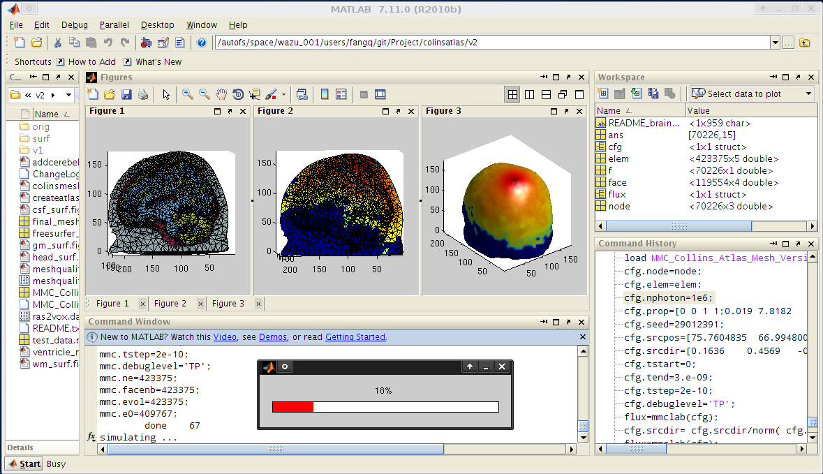
Screenshot for using MMCLAB in MATLAB:
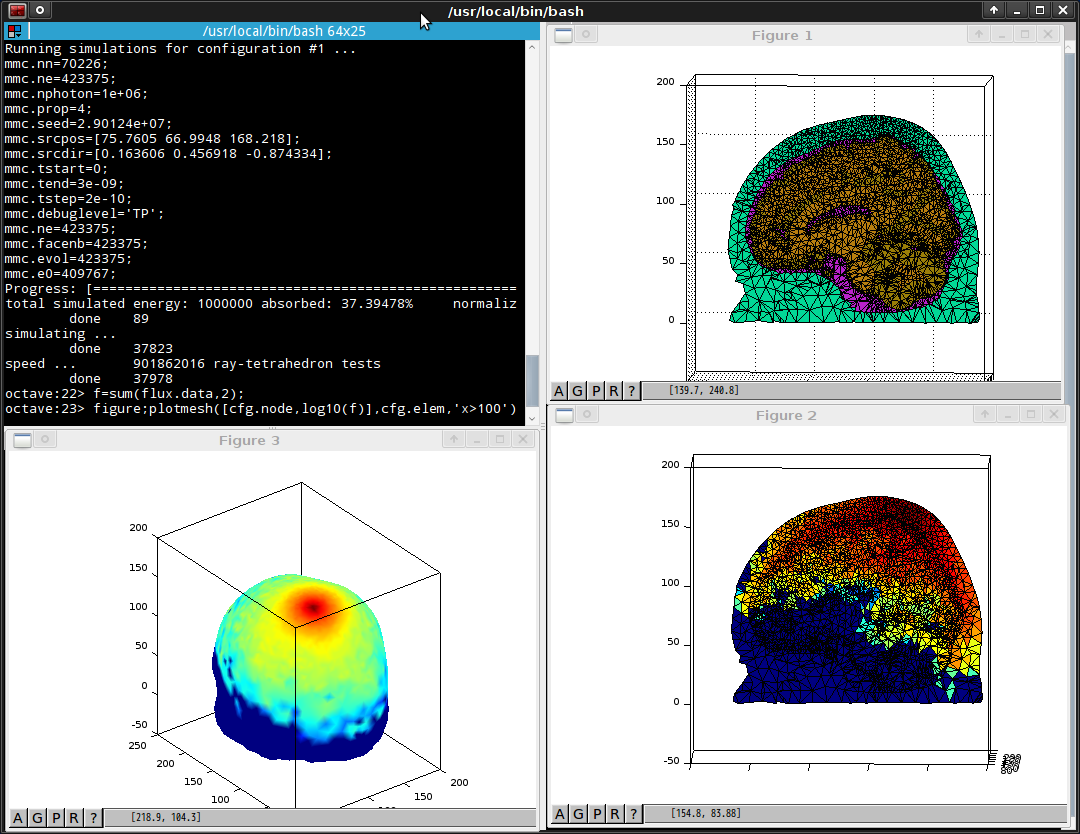
Screenshot for using MMCLAB in GNU Octave:
7. Reference
[Fang2010] Fang Q, "Mesh-based Monte Carlo method using fast ray-tracing in Plucker coordinates," Biomed. Opt. Express 1(1), 165-175 (2010)