![[Home]](/img/mcx_wiki_banner.png)
MCXLAB: MCX for MATLAB and GNU Octave
- Author: Qianqian Fang <q.fang at neu.edu>
- License: GNU General Public License version 3 (GPLv3)
- Version: this package is part of Monte Carlo eXtreme (MCX) v2019.2
- 1. Introduction
- 2. Installation
- 3. How to use MCXLAB in MATLAB/Octave
- 4. Examples
- 5. How to compile MCXLAB
- 6. Screenshots
- 7. Reference
1. Introduction
MCXLAB is the native MEX version of MCX for Matlab and GNU Octave. It compiles the entire MCX code into a MEX function which can be called directly inside Matlab or Octave. The input and output files in MCX are replaced by convenient in-memory struct variables in MCXLAB, thus, making it much easier to use and interact. Matlab/Octave also provides convenient plotting and data analysis functions. With MCXLAB, your analysis can be streamlined and speed- up without involving disk files.
Because MCXLAB contains the exact computational codes for the GPU calculations as in the MCX binaries, MCXLAB is expected to have identical performance when running simulations. By default, we compile MCXLAB with the support of recording detected photon partial path-lengths (i.e. the "make det" option). In addition, we also provide "mcxlab_atom": an atomic version of mcxlab compiled similarly as "make detbox" for MCX. It supports atomic operations using shared memory enabled by setting "cfg.sradius" input parameter to a positive number.
2. Installation
To download MCXLAB, please visit this link. If you choose to register, you will have an option to be notified for any future updates.
The system requirements for MCXLAB are the same as MCX: you have to make sure that you have a CUDA-capable graphics card with properly configured CUDA driver (you can run the standard MCX binary first to test if your system is capable to run MCXLAB). Of course, you need to have either Matlab or Octave installed.
Once you set up the CUDA toolkit and NVIDIA driver, you can then add the "mcxlab" directory to your Matlab/Octave search path using the addpath command. If you want to add this path permanently, please use the "pathtool" command, or edit your startup.m (~/.octaverc for Octave).
If everything works ok, typing "help mcxlab" in Matlab/Octave will print the help information. If you see any error, particularly any missing libraries, please make sure you have downloaded the matching version built for your platform.
3. How to use MCXLAB in MATLAB/Octave
To learn the basic usage of MCXLAB, you can type
help mcxlab
in Matlab/Octave to see the help information regarding how to use this function. The help information is listed below. You can find the input/output formats and examples. The input cfg structure has very similar field names as the verbose command line options in MCX.
 ====================================================================
       mcxlab - Monte Carlo eXtreme (MCX) for MATLAB/GNU Octave
 --------------------------------------------------------------------
 Copyright (c) 2011-2019 Qianqian Fang <q.fang at neu.edu>
                       URL: http://mcx.space
 ====================================================================

  Format:
     fluence=mcxlab(cfg);
        or
     [fluence,detphoton,vol,seed,trajectory]=mcxlab(cfg);
     [fluence,detphoton,vol,seed,trajectory]=mcxlab(cfg, option);

  Input:
     cfg: a struct, or struct array. Each element of cfg defines
          the parameters associated with a simulation.
          if cfg='gpuinfo': return the supported GPUs and their parameters,
          see sample script at the bottom
     option: (optional), options is a string, specifying additional options
          option='preview': this plots the domain configuration using mcxpreview(cfg)
          option='mcxcl':   this calls mcxcl.mex* instead of mcx.mex* on non-NVIDIA hardware


     cfg may contain the following fields:

 == Required ==
      *cfg.nphoton:    the total number of photons to be simulated (integer)
                       maximum supported value is 2^63-1
      *cfg.vol:        a 3D array specifying the media index in the domain.
                       can be uint8, uint16, uint32, single or double
                       arrays.
                       2D simulations are supported if cfg.vol has a singleton
                       dimension (in x or y); srcpos/srcdir must belong to
                       the 2D plane in such case.
                       for 2D simulations, Example: <demo_mcxlab_2d.m>
      *cfg.prop:       an N by 4 array, each row specifies [mua, mus, g, n] in order.
                       the first row corresponds to medium type 0
                       (background) which is typically [0 0 1 1]. The
                       second row is type 1, and so on. The background
                       medium (type 0) has special meanings: a photon
                       terminates when moving from a non-zero to zero voxel.
      *cfg.tstart:     starting time of the simulation (in seconds)
      *cfg.tstep:      time-gate width of the simulation (in seconds)
      *cfg.tend:       ending time of the simulation (in second)
      *cfg.srcpos:     a 1 by 3 vector, the position of the source in grid unit
      *cfg.srcdir:     a 1 by 3 vector, specifying the incident vector; if srcdir
                       contains a 4th element, it specifies the focal length of
                       the source (only valid for focuable src, such as planar, disk,
                       fourier, gaussian, pattern, slit, etc); if the focal length
                       is nan, all photons will be launched isotropically regardless
                       of the srcdir direction.

 == MC simulation settings ==
       cfg.seed:       seed for the random number generator (integer) [0]
                       if set to a uint8 array, the binary data in each column is used
                       to seed a photon (i.e. the "replay" mode)
                       Example: <demo_mcxlab_replay.m>
       cfg.respin:     repeat simulation for the given time (integer) [1]
                       if negative, divide the total photon number into respin subsets
       cfg.isreflect:  [1]-consider refractive index mismatch, 0-matched index
       cfg.bc          per-face boundary condition (BC), a strig of 6 letters for
                       bounding box faces at -x,-y,-z,+x,+y,+z axes;
 		               overwrite cfg.isreflect if given.
                       each letter can be one of the following:
                       '_': undefined, fallback to cfg.isreflect
                       'r': like cfg.isreflect=1, Fresnel reflection BC
                       'a': like cfg.isreflect=0, total absorption BC
                       'm': mirror or total reflection BC
                       'c': cyclic BC, enter from opposite face
       cfg.isnormalized:[1]-normalize the output fluence to unitary source, 0-no reflection
       cfg.isspecular: 1-calculate specular reflection if source is outside, [0] no specular reflection
       cfg.maxgate:    the num of time-gates per simulation
       cfg.minenergy:  terminate photon when weight less than this level (float) [0.0]
       cfg.unitinmm:   defines the length unit for a grid edge length [1.0]
                       Example: <demo_sphere_cube_subpixel.m>
       cfg.shapes:     a JSON string for additional shapes in the grid
                       Example: <demo_mcxyz_skinvessel.m>
       cfg.gscatter:   after a photon completes the specified number of
                       scattering events, mcx then ignores anisotropy g
                       and only performs isotropic scattering for speed [1e9]

 == GPU settings ==
       cfg.autopilot:  1-automatically set threads and blocks, [0]-use nthread/nblocksize
       cfg.nblocksize: how many CUDA thread blocks to be used [64]
       cfg.nthread:    the total CUDA thread number [2048]
       cfg.gpuid:      which GPU to use (run 'mcx -L' to list all GPUs) [1]
                       if set to an integer, gpuid specifies the index (starts at 1)
                       of the GPU for the simulation; if set to a binary string made
                       of 1s and 0s, it enables multiple GPUs. For example, '1101'
                       allows to use the 1st, 2nd and 4th GPUs together.
                       Example: <mcx_gpu_benchmarks.m>
       cfg.workload    an array denoting the relative loads of each selected GPU.
                       for example, [50,20,30] allocates 50%, 20% and 30% photons to the
                       3 selected GPUs, respectively; [10,10] evenly divides the load
                       between 2 active GPUs. A simple load balancing strategy is to
                       use the GPU core counts as the weight.
       cfg.isgpuinfo:  1-print GPU info, [0]-do not print

 == Source-detector parameters ==
       cfg.detpos:     an N by 4 array, each row specifying a detector: [x,y,z,radius]
       cfg.maxdetphoton:   maximum number of photons saved by the detectors [1000000]
       cfg.srctype:    source type, the parameters of the src are specified by cfg.srcparam{1,2}
                               Example: <demo_mcxlab_srctype.m>
                       'pencil' - default, pencil beam, no param needed
                       'isotropic' - isotropic source, no param needed
                       'cone' - uniform cone beam, srcparam1(1) is the half-angle in radian
                       'gaussian' [*] - a collimated gaussian beam, srcparam1(1) specifies the waist radius (in voxels)
                       'planar' [*] - a 3D quadrilateral uniform planar source, with three corners specified
                                 by srcpos, srcpos+srcparam1(1:3) and srcpos+srcparam2(1:3)
                       'pattern' [*] - a 3D quadrilateral pattern illumination, same as above, except
                                 srcparam1(4) and srcparam2(4) specify the pattern array x/y dimensions,
                                 and srcpattern is a floating-point pattern array, with values between [0-1].
                                 if cfg.srcnum>1, srcpattern must be a floating-point array with
                                 a dimension of [srcnum srcparam1(4) srcparam2(4)]
                                 Example: <demo_photon_sharing.m>
                       'pattern3d' [*] - a 3D illumination pattern. srcparam1{x,y,z} defines the dimensions,
                                 and srcpattern is a floating-point pattern array, with values between [0-1].
                       'fourier' [*] - spatial frequency domain source, similar to 'planar', except
                                 the integer parts of srcparam1(4) and srcparam2(4) represent
                                 the x/y frequencies; the fraction part of srcparam1(4) multiplies
                                 2*pi represents the phase shift (phi0); 1.0 minus the fraction part of
                                 srcparam2(4) is the modulation depth (M). Put in equations:
                                     S=0.5*[1+M*cos(2*pi*(fx*x+fy*y)+phi0)], (0<=x,y,M<=1)
                       'arcsine' - similar to isotropic, except the zenith angle is uniform
                                 distribution, rather than a sine distribution.
                       'disk' [*] - a uniform disk source pointing along srcdir; the radius is
                                set by srcparam1(1) (in grid unit)
                       'fourierx' [*] - a general Fourier source, the parameters are
                                srcparam1: [v1x,v1y,v1z,|v2|], srcparam2: [kx,ky,phi0,M]
                                normalized vectors satisfy: srcdir cross v1=v2
                                the phase shift is phi0*2*pi
                       'fourierx2d' [*] - a general 2D Fourier basis, parameters
                                srcparam1: [v1x,v1y,v1z,|v2|], srcparam2: [kx,ky,phix,phiy]
                                the phase shift is phi{x,y}*2*pi
                       'zgaussian' - an angular gaussian beam, srcparam1(0) specifies the variance in the zenith angle
                       'line' - a line source, emitting from the line segment between
                                cfg.srcpos and cfg.srcpos+cfg.srcparam(1:3), radiating
                                uniformly in the perpendicular direction
                       'slit' [*] - a colimated slit beam emitting from the line segment between
                                cfg.srcpos and cfg.srcpos+cfg.srcparam(1:3), with the initial
                                dir specified by cfg.srcdir
                       'pencilarray' - a rectangular array of pencil beams. The srcparam1 and srcparam2
                                are defined similarly to 'fourier', except that srcparam1(4) and srcparam2(4)
                                are both integers, denoting the element counts in the x/y dimensions, respectively.
                                For exp., srcparam1=[10 0 0 4] and srcparam2[0 20 0 5] represent a 4x5 pencil beam array
                                spanning 10 grids in the x-axis and 20 grids in the y-axis (5-voxel spacing)
                       source types marked with [*] can be focused using the
                       focal length parameter (4th element of cfg.srcdir)
       cfg.{srcparam1,srcparam2}: 1x4 vectors, see cfg.srctype for details
       cfg.srcpattern: see cfg.srctype for details
       cfg.srcnum:     the number of source patterns that are
                       simultaneously simulated; only works for 'pattern'
                       source, see cfg.srctype='pattern' for details
                       Example <demo_photon_sharing.m>
       cfg.issrcfrom0: 1-first voxel is [0 0 0], [0]- first voxel is [1 1 1]
       cfg.replaydet:  only works when cfg.outputtype is 'jacobian', 'wl', 'nscat', or 'wp' and cfg.seed is an array
                       -1 replay all detectors and save in separate volumes (output has 5 dimensions)
                        0 replay all detectors and sum all Jacobians into one volume
                        a positive number: the index of the detector to replay and obtain Jacobians
       cfg.voidtime:   for wide-field sources, [1]-start timer at launch, or 0-when entering
                       the first non-zero voxel

 == Output control ==
       cfg.issaveexit: [0]-save the position (x,y,z) and (vx,vy,vz) for a detected photon
                       Example: <demo_lambertian_exit_angle.m>
       cfg.issaveref:  [0]-save diffuse reflectance/transmittance in the non-zero voxels
                       next to a boundary voxel. The reflectance data are stored as
                       negative values; must pad zeros next to boundaries
                       Example: see the demo script at the bottom
       cfg.outputtype: 'flux' - fluence-rate, (default value)
                       'fluence' - fluence integrated over each time gate,
                       'energy' - energy deposit per voxel
                       'jacobian' or 'wl' - mua Jacobian (replay mode),
                       'nscat' or 'wp' - weighted scattering counts for computing Jacobian for mus (replay mode)
                       for type jacobian/wl/wp, example: <demo_mcxlab_replay.m>
                       and  <demo_replay_timedomain.m>
       cfg.session:    a string for output file names (only used when no return variables)

 == Debug ==
       cfg.debuglevel:  debug flag string, one or a combination of ['R','M','P'], no space
                     'R':  debug RNG, output fluence.data is filled with 0-1 random numbers
                     'M':  return photon trajectory data as the 5th output
                     'P':  show progress bar
       cfg.maxjumpdebug: [10000000|int] when trajectory is requested in the output,
                      use this parameter to set the maximum position stored. By default,
                      only the first 1e6 positions are stored.

       fields with * are required; options in [] are the default values

  Output:
       fluence: a struct array, with a length equals to that of cfg.
             For each element of fluence, fluence(i).data is a 4D array with
             dimensions specified by [size(vol) total-time-gates].
             The content of the array is the normalized fluence at
             each voxel of each time-gate.
       detphoton: (optional) a struct array, with a length equals to that of cfg.
             Starting from v2018, the detphoton contains the below subfields:
               detphoton.detid: the ID(>0) of the detector that captures the photon
               detphoton.nscat: cummulative scattering event counts in each medium
               detphoton.ppath: cummulative path lengths in each medium (partial pathlength)
                    one need to multiply cfg.unitinmm with ppath to convert it to mm.
               detphoton.mom: cummulative cos_theta for momentum transfer in each medium
               detphoton.p or .v: exit position and direction, when cfg.issaveexit=1
               detphoton.w0: photon initial weight at launch time
               detphoton.prop: optical properties, a copy of cfg.prop
               detphoton.data: a concatenated and transposed array in the order of
                     [detid nscat ppath mom p v w0]'
               "data" is the is the only subfield in all mcxlab before 2018
       vol: (optional) a struct array, each element is a preprocessed volume
             corresponding to each instance of cfg. Each volume is a 3D int32 array.
       seeds: (optional), if give, mcxlab returns the seeds, in the form of
             a byte array (uint8) for each detected photon. The column number
             of seed equals that of detphoton.
       trajectory: (optional), if given, mcxlab returns the trajectory data for
             each simulated photon. The output has 6 rows, the meanings are
                id:  1:    index of the photon packet
                pos: 2-4:  x/y/z/ of each trajectory position
                     5:    current photon packet weight
                     6:    reserved
             By default, mcxlab only records the first 1e7 positions along all
             simulated photons; change cfg.maxjumpdebug to define a different limit.


  Example:
       % first query if you have supported GPU(s)
       info=mcxlab('gpuinfo')

       % define the simulation using a struct
       cfg.nphoton=1e7;
       cfg.vol=uint8(ones(60,60,60));
       cfg.vol(20:40,20:40,10:30)=2;    % add an inclusion
       cfg.prop=[0 0 1 1;0.005 1 0 1.37; 0.2 10 0.9 1.37]; % [mua,mus,g,n]
       cfg.issrcfrom0=1;
       cfg.srcpos=[30 30 1];
       cfg.srcdir=[0 0 1];
       cfg.detpos=[30 20 1 1;30 40 1 1;20 30 1 1;40 30 1 1];
       cfg.vol(:,:,1)=0;   % pad a layer of 0s to get diffuse reflectance
       cfg.issaveref=1;
       cfg.gpuid=1;
       cfg.autopilot=1;
       cfg.tstart=0;
       cfg.tend=5e-9;
       cfg.tstep=5e-10;
       % calculate the fluence distribution with the given config
       [fluence,detpt,vol,seeds,traj]=mcxlab(cfg);

       % integrate time-axis (4th dimension) to get CW solutions
       cwfluence=sum(fluence.data,4);  % fluence rate
       cwdref=sum(fluence.dref,4);     % diffuse reflectance
       % plot configuration and results
       subplot(231);
       mcxpreview(cfg);title('domain preview');
       subplot(232);
       imagesc(squeeze(log(cwfluence(:,30,:))));title('fluence at y=30');
       subplot(233);
       hist(detpt.ppath(:,1),50); title('partial path tissue#1');
       subplot(234);
       plot(squeeze(fluence.data(30,30,30,:)),'-o');title('TPSF at [30,30,30]');
       subplot(235);
       newtraj=mcxplotphotons(traj);title('photon trajectories')
       subplot(236);
       imagesc(squeeze(log(cwdref(:,:,1))));title('diffuse refle. at z=1');

  This function is part of Monte Carlo eXtreme (MCX) URL: http://mcx.space

  License: GNU General Public License version 3, please read LICENSE.txt for details
4. Examples
We provided several examples to demonstrate the basic usage of MCXLAB, as well as to perform validations of MCX algorithm using both simple homogeneous and heterogeneous domains. These examples are explained below:
demo_mcxlab_basic.m
In this example, we show the most basic usage of MCXLAB. This include how to define the input configuration structure, launch MCX simulations and interpret and plotting the resulting data.
demo_validation_homogeneous.m
In this example, we validate MCXLAB with a homogeneous medium in a cubic domain. This is exactly the example shown in Fig.5 of [Fang2009].
You can also use the alternative optical properties that has a high g value to observe the similarity between the two scattering/g configurations.
demo_validation_heterogeneous.m
In this example, we validate the MCXLAB solver with a heterogeneous domain and the analytical solution of the diffusion model. We also demonstrate how to use sub-pixel resolution to refine the representation of heterogeneities. The domain is consisted of a 6x6x6 cm box with a 2cm diameter sphere embedded at the center.
This test is identical to that used for Fig. 3 in [Fang2010].
demo_sphere_cube_subpixel.m
In this example, we demonstrate how to use sub-pixel resolution to represent the problem domain. The domain is consisted of a 6x6x6 cm box with a 2cm diameter sphere embedded at the center.
demo_4layer_head.m
In this example, we simulate a 4-layer brain model using MCXLAB. We will investigate the differences between the solutions with and witout boundary reflections (both external and internal) and show you how to display and analyze the resulting data.
demo_mcxlab_srctype.m
This demo script shows how to use 9 different types sources in your simulations. These 9 source types include pencil beam, isotropic source, Gaussian beam, uniform plannar source, uniform disk source, Fourier pattern illumuniation (spatial frequency domain sources), arcsine distribution beam, uniform cone beam, and an arbitrary light pattern (defined by a 2D image).
bench_reseedlimit.m
In this simulation, we verify the reduction of Monte Carlo stochastic noise with respect to the increase of photon numbers. We also test the effect of the reseedlimit parameter and its impact to the noise.
5. How to compile MCXLAB
To compile MCXLAB for Matlab, you need to cd mcx/src directory, and type
make mex
from a shell window. You need to make sure your Matlab is installed and the command mex is included in your PATH environment variable. Similarly, to compile MCXLAB for Octave, you type
make oct
The command mkoctfile must be accessible from your command line and it is provided in a package named "octave3.x-headers" in Ubuntu (3.x can be 3.2 or 3.4 etc).
If your graphics card is a Fermi-class or newer, you can compile MCXLAB with make fermimex or fermioct. The output mex file can determine the level of atomic operations using the cfg.sradius settings.
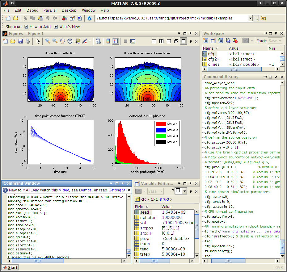
6. Screenshots
Screenshot for using MCXLAB in Matlab:
Screenshot for using MCXLAB in GNU Octave:

7. Reference
 [Yu2018] Leiming Yu, Fanny Nina-Paravecino, David Kaeli, Qianqian Fang,
 "Scalable and massively parallel Monte Carlo photon transport simulations
 for heterogeneous computing platforms," J. Biomed. Opt. 23(1), 010504 (2018).
 [Fang2009] Qianqian Fang and David A. Boas, "Monte Carlo simulation
  of photon migration in 3D turbid media accelerated by graphics processing
  units," Opt. Express 17, 20178-20190 (2009)